Planet Georezo » Planet OSGeo

Un Planet est un site Web dynamique qui agrÃ¨ge le plus souvent sur une seule page, le contenu de notes, d'articles ou de billets publiÃ©s sur des blogs ou sites Web afin d'accentuer leur visibilitÃ© et de faire ressortir des contenus pertinents aux multiples formats (texte, audio, vidÃ©o, Podcast). C'est un agrÃ©gateur de flux RSS. Il s'apparente Ã un portail web.
Vous pouvez lire le billet sur le blog La Minute pour plus d'informations sur les RSS !

Canaux

3531 éléments (4 non lus) dans 55 canaux

Dans la presse

Du côté des éditeurs

Toile géomatique francophone

Géomatique anglophone

Blogs GeoRezo.net

Abonnez vous à cette page (RSS) !

Planet OSGeo

Sauter à la page: 1 2 3 ... 6

24 July 2024
13:40
WhereGroup: Erweiterte Geodatenvisualisierung mit MapComponents
sur Planet OSGeo

Die MapComponents-Bibliothek ermöglicht die Anzeige und Integration verschiedener Datenformate direkt im Browser. Anhand eines praktischen Beispiels wird gezeigt, wie Benutzer OpenStreetMap-Daten in eine Webanwendung laden und diese anzeigen lassen können.
11:00
Mappery: Coaster
sur Planet OSGeo

A classic but always good from Chris Chambers.
MapsintheWild Coaster
23 July 2024
11:15
Jorge Sanz: Elastic Volunteering Time Off
sur Planet OSGeo

My employer, Elastic, has a number of philanthropic initiatives but definitely the one I love the most is the Volunteering Time Off (VTO). We are given 40 hours per year from our working hours to contribute to projects and initiatives we care about. Employees have full freedom to choose what they want to do with that time and are encouraged to use it.

In my case, over this almost 5 years I have to admit I haven’t used all that time every year but I tried to get the most of it. During COVID I did some remote work for a local NGO that works for fair trade, giving them a webinar about Open Source among other things (see update from December 2019 and following months). I also spent a few days working on some admin tasks for the Open Source Geospatial Foundation and I’ve already written here about a couple sessions I did for Cibervoluntarios, training seniors and teens about safe browsing and email.

Last week I was showcased in the company blog, along with other colleagues, on different projects to contribute to. In my case, last year I joined the mapping efforts after the Morocco Earthquake and took a full day mapping roads and streets of a rural area, as part of the coordinated efforts from the Humanitarian OpenStreetMap team (reported on my October community update). I’m very happy to have this support from my employer to leave things aside when an emergency like this arises, granted there are no other urgent issues at work.

As a personal call to action, I’d love to get back to Cibervoluntarios activities. This year has been quite busy; let’s see after summer if there’s room for getting out and engaging with them.

I know I haven’t updated this site in a while, I’ll write one soon! ?

Reply by mail or from the fediverse
11:00
Mappery: Geodesic point
sur Planet OSGeo

Jilles van Gurp shared this geodesic point in Hannover with us.
MapsintheWild Geodesic point
9:00
QGIS Blog: Introducing the new QGIS.org website
sur Planet OSGeo
We have a new website!

We recently launched our new website at QGIS.org. It is a ground-up overhaul and provides a fresh take on the first contact point for existing or potential users wishing to engage with the QGIS project and discover its value proposition.

A new strategy for QGIS.org websites

In this blog post, we would like to provide an overview of the goals that we had for building the new QGIS.org website and the bigger picture of how this website update fits into the broader strategy for our website plans for QGIS.

About two years ago, we started experimenting with building a new QGIS.org website based on Hugo. Hugo, as a technology choice, was less important than was our intent to develop a more modern site that addressed our strategic goals.

After some ‘in-house’ (i.e. volunteer-based) work to develop an initial version of the site, we received the go-ahead to use QGIS funds for this and put out a call in October 2023 for a company to support our work. This was ultimately won by Kontur.io, who, together with our volunteers, brought the work into high gear.
Initial analysis of the questions and actions to be quickly answered by qgis.org

Goal 1: Speak to a new audience

Our primary goal was to speak to a new audience. We are confident that QGIS can compete with all of the commercial vendors providing GIS software. We didn’t convey that well on our old website. We feel that QGIS was too apologetic in how it presented itself. We wanted a website which inspires confidence while addressing the needs of a corporate or organisational decision-maker who is looking at the QGIS project during their GIS software selection process.

The old website was very focused on the developer and contributor community. Obviously, those aspects are important since, without our fantastic community, the QGIS project would not exist. The messaging around open source is also important. Yet these ideas are secondary to the idea that QGIS is one of the best (if not the best) desktop GIS applications out there on the market – open-source or otherwise. We need to present it in this professional perspective.

So, the first goal was to change the messaging to focus on QGIS’s value proposition and take a very professional approach to presenting ourselves on the website.
User group and requirements analysis for the potential qgis.org visitors

Goal 2: Harmonisation

The second goal was to start the process of harmonising all of our website properties. QGIS.org, over the years, has built many different web properties. For example, there’s the plugins website, the feed, the changelog, the sustaining members website, the lessons website and the certification website, the new resources hub website, the API documentation, the user documentation, the user manual, the training manual, various other documentation efforts, and more. Some of those are combined in one application, There are also some less well-known resources, like our analytics.qgis.org and another one for plugin analytics. In short, we’ve a lot of resources!

With so many different web properties, they’ve devolved over time: each has its own look and feel, navigation approach and how you interact with it. Some of them were translated, and some of them were not. We want to harmonise all of these sites so that the user does not notice any change in user experience when they move from one QGIS-related site to another.

Goal 3: Harmonising deployment

In the underlying process of these changes, we’re also redeploying all of the websites on new servers, which are more up-to-date and use better security and maintenance practices. Plenty of work is happening in the background to ensure that all of the servers are in a better-maintained state, document how they’re maintained, and so on.

Goal 4: A hub and spokes

The objective of the new site design is to allow quick movement between the QGIS auxiliary sites. The QGIS.org site will form a hub that effortlessly takes visitors to whichever QGIS-related site they need to complete the task they are busy with. If you’re moving between these sites, the experience should be seamless. You should not really even be aware that you’re moving between different websites. Other than looking at the URL bar, the user presentation and experience should be harmonious between all of them.

One way we are planning to achieve this is to have a universal menu bar and footer. You will see that in the new website’s design, there is a menu bar across the top. This menu bar has two levels: the top menu and the second level, where the search bar is.
The universal menu bar
In this second row, auxiliary sites will have their own sub-menu whilst keeping the shared top-level menu. So if you, for example, are moving around in plugins and want to review the plugin list or submit a new plugin, all of that navigation will be on the second line where the search bar is currently. Regardless of which subdomain you are on, the top-level menu bar will be the same, allowing you to easily navigate back to the hub or to another subdomain.

The footer will be unified and shared between all sites, and the cascading style sheets and styling will be unified across all of the QGIS websites.

In the next phase, we will work to achieve this coherence across all the websites, though we still have a few more tweaks to make to the qgis.org site first.

Goal 5: DOTDOTW – do one thing, do one thing well

We plan to break some auxiliary websites apart into separate pieces. So, for example, the changelog management, certification management, sustaining members management, and lessons management are all in one Django app. We will split them into small single-purpose applications using some common UX metaphors so that each is a standalone application that makes it easy for a potential contributor to understand everything the application does. This will also simplify management as we can upgrade each auxiliary site on separate development cycles. We will also finally have semantic URLs, e.g. certification.qgis.org, to take you to the different areas of interest on the site.

The plugins.qgis.org is also going to be refactored so that it just has plugins and not the resource sharing we’ve added in the last few years. The resource sharing will go into its own subdomain. Similarly, the Planet website will get split into its own website (the planet is a blog aggregator or RSS aggregator) that will be in its own managed instance. Some other components (like the analytics) are difficult to split out like this because they’re linked to the same database. We will try to make sure that those are more discoverable and theme them as much as possible to match the rest of the website experience.

Goal 7: Encapsulation

Another goal we had for the QGIS.org makeover was to make the site performant and self-contained. By self-contained, we mean that it should not ‘call’ out to CDN, Google or other platforms for resources like fonts, CSS frameworks, javascript libraries, etc. There were two reasons for this:
1. These platforms often use such resources to track users as they move around the Internet, which we want to avoid as much as possible.
2. We want to wholly manage our site, be able to fix any issues independently and generally follow a path of self-determination.
Our approach also facilitated the creation of a very performant website, as you can see here. We will try to adhere to these principles for the auxiliary site updates we do in the future, too.
What about translations?
The question has come up: Why did we not want to translate the new QGIS.org when it was translated before?

Firstly, we should make it clear that we do not plan to remove translations from the user documentation, the user manual, and so on, where we think they have the most value.

For the main QGIS.org site, we question whether there is a high value in translating it. Here are some reasons why:

1. Lingua franca: If you are an IT manager in a non-English-speaking country and you want to evaluate some software, you’re going to run into a product page that presents itself in English – it is the norm for IT procurement to work in English for reviewing software products and so on.

2. Automation: Automated translations inside browsers are getting better and better. While these translations are still not completely adequate, we think they will be in one or two years’ time.

3. Translation integrity: Our pursuit of Goal 1 means that we would no longer find it acceptable to have partial website translations. We also need to ensure that the wording and phrasing are consistent with the English messaging. We also have concerns about the QA process regarding trust and review – we want to ensure that any translation truly reflects the meaning and intent of the original content and has not been adjusted during the translation process.

4. Cohesion: Our most important point is raised if we go back to this idea of cohesion between the different websites like QGIS.org, plugins.qgis.org and so on. As well as having the same styling, we also don’t want to switch between languages as you hop between the sites. We aim to present them all as one site. If we translate QGIS.org and then take you to our auxiliary sites, e.g., plugins.qgis.org, the feed, or certification pages, which are in English only, the experience is jarring.

So we must either translate everything into all of the same languages, or work in English. Translating everything is a mammoth task for the translators and for us to retrospectively add translation support to each platform. Thus, we prefer the approach of harmonising everything to one language and then focusing our translation efforts on three areas:
1. The application itself,
2. the user manual and
3. the training manuals.
We can leave the rest of the experience in English and instead focus on harmonising, for now, both in terms of look and feel and the technology used.

When we consider everything as one big website and what the bigger plan is, it is hopefully clearer why we didn’t think translating the landing page and QGIS.org was the best approach.
Further funded work
We hope to use more QGIS funding to support this work in the future. We’re also hoping to work again with Kontur to start moving all these auxiliary sites into their own projects, applying our style guidelines to each. Independently of that, Tim (volunteer), Lova (QGIS funded), and others are already getting started with this process.
Helping out
Do you have strong opinions about the website? Contact Tim on the PSC mailing list if you would like to get involved as a volunteer. We would love to hear from designers, word smiths, marketers, information architects, SEO specialists, web developers and those who think they can help us achieve our goals.
Conclusion
We hope our goals and process make sense for everybody and that we were able to lay out a clear, logical argument about why we don’t want to translate the new website quite yet. We want to focus on these overarching goals and then return to them later if they are still a priority for people. Everything we have built is Open Source and available at this repo, where you can also find an issue tracker to report issues and share ideas relating to the new website.

Thanks for reading. Go spatial without compromise

Cheers, Tim, Marco and Anita
2:00
SourcePole: Adding external WMS to the QGIS Cloud Web Map
sur Planet OSGeo

The use of WMS/WMTS layers in a QGIS Cloud map project can significantly degrade the performance of the map display. I have already discussed how to counter this problem in an earlier post. One of the solutions is to load external WMS as background layers. The problem with this approach, however, is that only one WMS background layer can be loaded at a time. If further WMS layers are to be loaded into the map at the same time, this approach cannot be used.
22 July 2024
11:00
Mappery: Wallpaper
sur Planet OSGeo

Chris Chambers shared this wallpaper.
MapsintheWild Wallpaper
2:00
GeoServer Team: GeoServer 2024 Q3 Developer Update
sur Planet OSGeo
This is a follow up to 2024 roadmap post outlining development opportunities.

First of all thanks to developers and organisations that have responded with offers of in-kind contributions. This blog post is assessing current progress and outlines a way forward to complete the Java 17/Jakarta EE/Spring 6 upgrades.

This post highlights development activities that are available to be worked on today, along with interested developers and commercial support providers available to work on GeoServer roadmap items.
Spring Framework 6 Tasks
The key challenge we are building towards is a spring-framework 6 update, ideally by the end of 2024 when the version we use now reaches end-of-life.

The tasks below are steps towards this goal.
Wicket 9 upgrade
Interested Parties:
- Brad has been doing amazing work with the Wicket 9 upgrade and is in need of assistance.
- GeoCat has offered to do manual A/B testing when PR is ready for testing.
Activity:
- [GEOS-11275] Wicket 9 upgrade
- geoserver#7154
Spring Security 5.8 update
Spring Security 5.8 provides a safe stepping stone ahead of the complete spring-framework 6 upgrade and is an activity that can be worked on immediately.

Interested parties:
- Andreas Watermeyer (ITS Digital Solutions) offered to work on this activity in during the initial January call out, and has indicated they are now ready to start.
Activity:
- [GEOS-11271] Upgrade spring-security to 5.8
Spring Security Core implementation of OAuth2 / OIDC
The spring-security-oauth client has reached end-of-life and a GeoServer OAuth2 support must be rewritten or migrated as a result.

There are two paths to migrate to spring-security-core implementation:
- Option: Migrate the existing community module implementations to spring-security-core in place; with as little loss of functionality as possible. This has the advantage of using existing test coverage to maintain a consistent set of functionality during migration.
- Option: Setup a community module alongside the existing implementation with the goal of making a full supported etension. This approach has the advantages of allowing organisations the ability to do A/B testing as both the old and new implementation would be available alongside each other. This has the advantage of allowing stakeholders to only fund, implement, test functionality as required without disrupting existing use.
Security integrations often require infrastructure to develop and test against, which the core GeoServer team does not have access to for automated tests. We would like to see organisations review their security integration requirements and be on hand to support this development activity.

The initial priority will support for OAuth2 and Open ID Connect (OIDC), parties interested in maintaining support for Google, GeoNode, GitHub are welcome to participate.

Interested Parties:
- Andreas Watermeyer (ITS Digital Solutions) offered to work on this activity, or test as needed.
- GeoCat is interested in this work also, with the goal of bringing the OIDC plugin up to full extension status (if financing is available).
Activity: not started
- [GEOS-11272] spring-security-oauth replacement, with spring-security 5.8
ImageN / JAI Replacement
The image processing library used by GeoServer has been donated to the open source community under the name ImageN.

The immediate goal has been to add test cases to this codebase and make an ImageN 1.0 release. Andrea has come up with the amazing idea of integrating with JAI-Ext project immediately, to benefit from the improved operators, and jumpstart test coverage.

Interested Parties:
- Jody (GeoCat) is available to support this activity, or take lead if funding is available.
- Andrea (GeoSolutions) has had a deep dive into the implications for the JAI-EXT project outlining a roadmap for project integration
We would like to see organisations that depend on GeoServer for earth observation and imagery to step forward with funding for this activity.
2024 Financial support and sponsorship
Thus far 2024 has not had a strong enough sponsorship response to support the project goals above. As a point of comparison we established a budget of $15,000 with OSGeo last year to take on an low-level API change that affected several projects.

This year GeoServer sponsorship has raised between $1,000 and $2,000 which is not enough to plan with or coordinate in-kind contributions offered thus far.

Jody has worked with the OSGeo board to make adjustments to the sponsorship:
- Guidance has been provided for appropriate sponsorship levels for individual consultants, small organisation, companies and public institutions of different sizes.
- There are clear examples of how to sponsor and donate, along with the the perks and publicity associated with financial support
- GeoServer has a new sponsorship page on our website collecting this information
- GeoServer now lists sponsors logos on our home page, alongside core contributors.
We would like to thank everyone who has responded thus far:
- Sponsors: How 2 Map, illustreets
- Individual Donations: Peter Rushforth, Marco Lucarelli, Gabriel Roldan, Jody Garnett, Manuel Timita, Andrea Aime
21 July 2024
13:00
From GIS to Remote Sensing: Semi-Automatic Classification Plugin version 8.3 release date
sur Planet OSGeo

This post is to announce that the new version 8.3 of the Semi-Automatic Classification Plugin (SCP) for QGIS will be released the 3rd of August 2024.This new version will require the new version 0.4 of the Python processing framework Remotior Sensus, and will include several new features such as such as clustering, raster editing and raster zonal stats.

For any comment or question, join the Facebook group or GitHub discussions about the Semi-Automatic Classification Plugin.
11:00
Mappery: Which projection is this?
sur Planet OSGeo

I found this nice geo license plate walking by the River Thames. Very geo-nerdy. Happy Sunday!
MapsintheWild Which projection is this?
20 July 2024
15:41
From GIS to Remote Sensing: Remotior Sensus Update: Version 0.4
sur Planet OSGeo
I'm glad to announce the update of Remotior Sensus to version 0.4.This new version add several new features such as clustering, raster editing and raster zonal stats. Following the complete changelog:
- Added tool "Band clustering" for unsupervised K-means classification of bandset
- Added tool "Raster edit" for direct editing of pixel values based on vector
- Added tool "Raster zonal stats" for calculating statistics of a raster intersecting a vector.
- Improved the NoData handling for multiprocess calculation
- In "Band clip", "Band dilation", "Band erosion", "Band sieve", "Band neighbor", "Band resample" added the option multiple_resolution to keep original resolution of individual rasters, or use the resolution of the first raster for all the bands
- In "Cross classification" fixed area based accuracy and added kappa hat metric
- In "Band combination" added option no_raster_output to avoid the creation of output raster, producing only the table of combinations
- In "Band calc" replaced nanpercentile with optimized calculation function
- Improved extraction of ROIs in "Band classification"
- Minor bug fixing and removed Requests dependency
Read more »
11:00
Mappery: Corsica
sur Planet OSGeo

This charcuterie platter is in Corsica’s shape.
MapsintheWild Corsica
19 July 2024
17:43
GeoNode: Docs For Devs
sur Planet OSGeo

GeoNode: Docs For Devs
17:43
GeoNode: Translate
sur Planet OSGeo

GeoNode: Translate
17:43
GeoNode: Improve
sur Planet OSGeo

GeoNode: Improve
17:43
GeoNode: Future
sur Planet OSGeo

GeoNode: Future
17:43
GeoNode: Patches
sur Planet OSGeo

GeoNode: Patches
17:43
GeoNode: Contribute
sur Planet OSGeo

GeoNode: Contribute
17:43
GeoNode: Extend
sur Planet OSGeo

GeoNode: Extend
17:43
GeoNode: Arch
sur Planet OSGeo

GeoNode: Arch
17:43
GeoNode: Testing
sur Planet OSGeo

GeoNode: Testing
17:43
GeoNode: Env Dev
sur Planet OSGeo

GeoNode: Env Dev
17:43
GeoNode: Management Commands
sur Planet OSGeo

GeoNode: Management Commands
17:43
GeoNode: Backups
sur Planet OSGeo

GeoNode: Backups
17:43
GeoNode: Other Languages
sur Planet OSGeo

GeoNode: Other Languages
17:43
GeoNode: Ssl
sur Planet OSGeo

GeoNode: Ssl
17:43
GeoNode: Troubleshoot
sur Planet OSGeo

GeoNode: Troubleshoot
17:43
GeoNode: Customize Geonode
sur Planet OSGeo

GeoNode: Customize Geonode
17:43
GeoNode: Production Geonode
sur Planet OSGeo

GeoNode: Production Geonode
17:43
GeoNode: Install Geonode
sur Planet OSGeo

GeoNode: Install Geonode
17:43
GeoNode: Share Map
sur Planet OSGeo

GeoNode: Share Map
17:43
GeoNode: Find Map
sur Planet OSGeo

GeoNode: Find Map
17:43
GeoNode: Create Map
sur Planet OSGeo

GeoNode: Create Map
17:43
GeoNode: Add Data
sur Planet OSGeo

GeoNode: Add Data
17:43
GeoNode: New Account
sur Planet OSGeo

GeoNode: New Account
17:43
GeoNode: Tutorials
sur Planet OSGeo

GeoNode: Tutorials
14:27
GeoTools Team: GeoTools 31.3 released
sur Planet OSGeo

 GeoTools 31.3 released The GeoTools team is pleased to announce the release of the latest maintenance version of  GeoTools 31.3: geotools-31.3-bin.zip geotools-31.3-doc.zip geotools-31.3-userguide.zip geotools-31.3-project.zip This release is also available from the  OSGeo Maven Repository and is made in conjunction with GeoServer 2.25.3  We
13:17
Adam Steer: Mapping a small farm part 3: using an aerial orthophoto
sur Planet OSGeo

Part 1 of this series looked at how to fly drones and collect imagery for mapping over a small property. Part 2 showed use cases for a digital elevation model. This story focusses on the georeferenced imagery produced in the process. It will look at three use cases – and explain some of the limitations:… Read More »Mapping a small farm part 3: using an aerial orthophoto
11:00
Mappery: Armchair
sur Planet OSGeo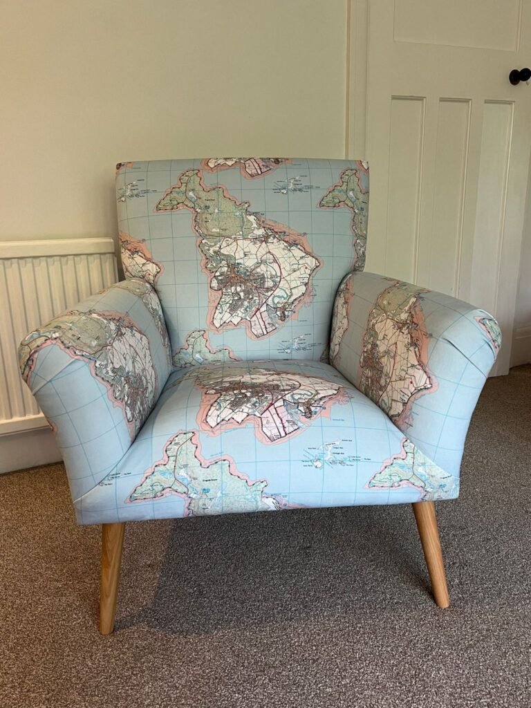

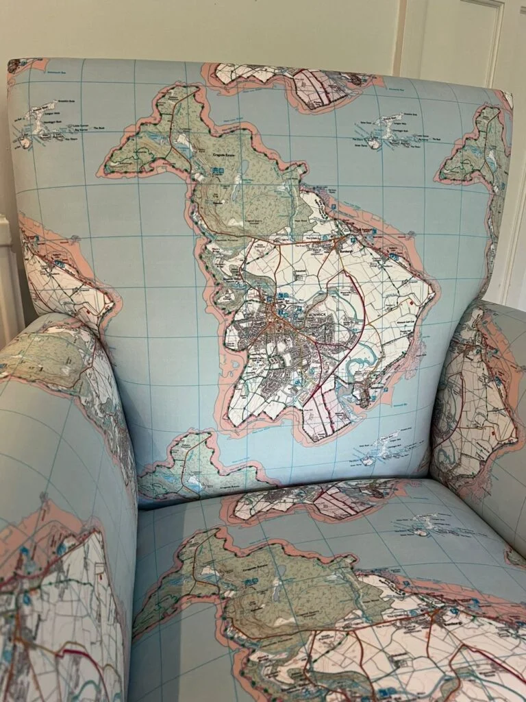
It is a bit unusual, but we found this one on LinkedIn. Chris Chambers received this armchair as a birthday gift.
MapsintheWild Armchair
2:00
Camptocamp: Optimizing Trail Management: Mergin Maps for Greater Annecy
sur Planet OSGeo

Pièce jointe: [télécharger]

Grand Annecy turned to Camptocamp to find the tool best suited to their needs.
17 July 2024
19:47
SIG Libre Uruguay: Va una más…
sur Planet OSGeo

edición 2024 del concurso: Proyectos de Geografía con estudiantes y gvSIG Batoví
19:45
gvSIG Batoví: edición 2024 del concurso: Proyectos de Geografía con estudiantes y gvSIG Batoví
sur Planet OSGeo

Habiendo finalizado con éxito la etapa de capacitación de la iniciativa Geoalfabetización mediante la utilización de Tecnologías de la Información Geográfica, lanzamos la convocatoria a participar de la edición 2024 del concurso: Proyectos de Geografía con estudiantes y gvSIG Batoví. Organizan Ceibal, la Dirección Nacional de Topografía del Ministerio de Transporte y Obras Públicas (MTOP), la Inspección Nacional de Geografía y Geología de la Dirección General de Educación Secundaria (DGES), junto con la Universidad Politécnica de Madrid (UPM). Pueden acceder aquí a la convocatoria y bases.

Este año contamos con la colaboración de la Dirección General de Educación Técnica Profesional (DGETP), la Asociación Nacional de Profesores de Geografía (ANPG) y la Universidad Central “Marta Abreu” de Las Villas (Cuba).

Agradecemos el apoyo de todas las instituciones que hacen posible la realización de esta propuesta.
11:00
Mappery: The Cure for Anything is Salt Water
sur Planet OSGeo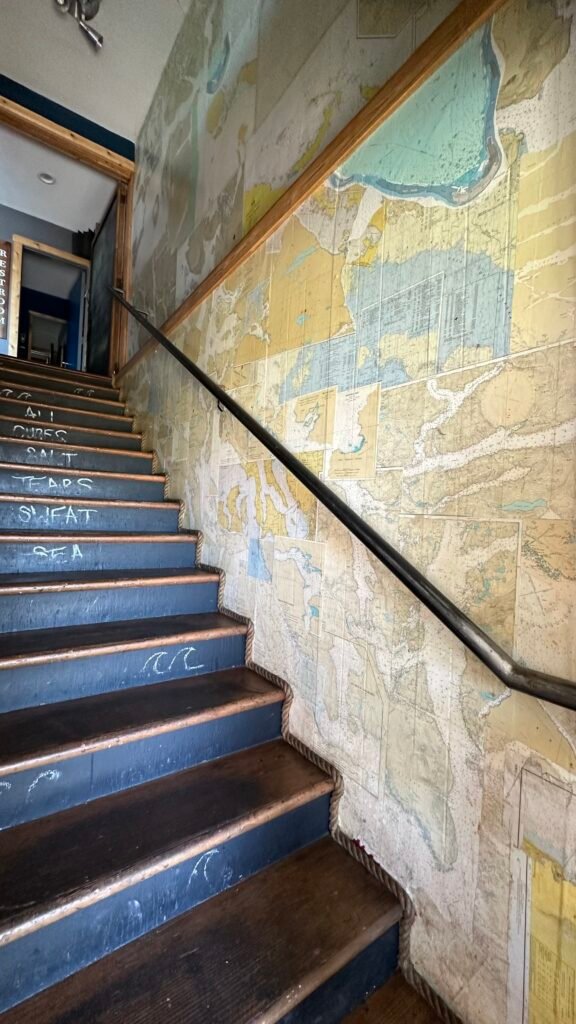

Darrell Fuhriman sent me these pics from the Salt Pub in Ilwaco, Washington.

“They decorated with old nautical charts, including a lamp shade and wallpaper on the stairs and entryway. “

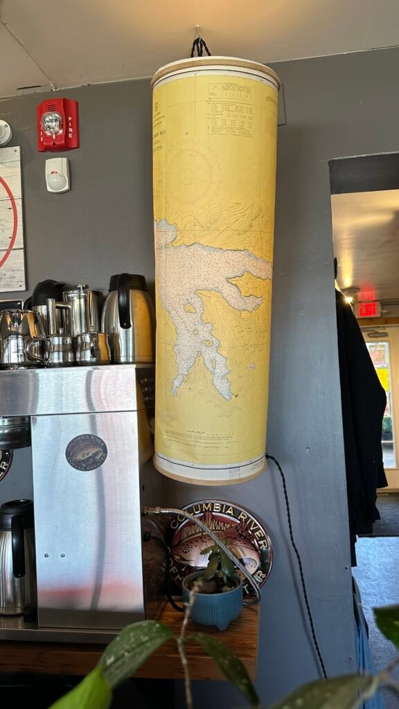
The stairs reference a quote by author Isak Dinesen. “The cure for anything is salt water — sweat, tears, or the sea.”

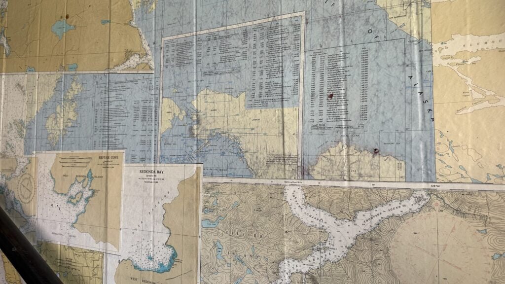
MapsintheWild The Cure for Anything is Salt Water
16 July 2024
14:34
GeoSolutions: FOSS4G North America: GeoSolutions Sponsoring FOSS4GNA – Workshops, and Presentations
sur Planet OSGeo

You must be logged into the site to view this content.
11:00
Mappery: Origin of the Species
sur Planet OSGeo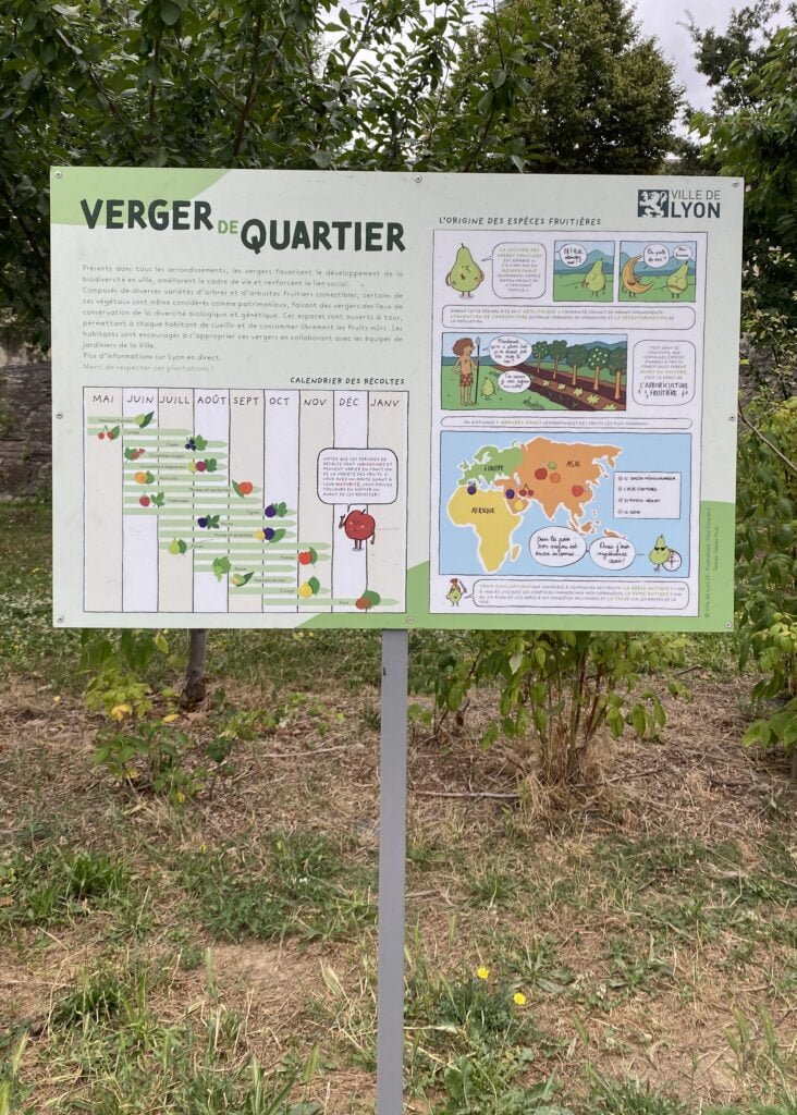

Reinder took this pic in a neighbourhood orchard “. along the river Saône in Lyon, named after a local heroine Mere Guy”

“In the 2nd arrondissement, the orchard created at Place Général Delfosse was named in honor of Mere Guy. A pioneer of the Meres de Lyon, she opened her restaurant in 1759 on the banks of the Rhône at Mulatière. She serves fish provided by her husband, a traditional fisherman, including her signature dish: eel matelote.” (Apologies for my translation)
[https:]

The map shows the origins of the various species in the orchard
MapsintheWild Origin of the Species
7:10
Adam Steer: Mapping a small farm part 2: microhydrology
sur Planet OSGeo

This is the first sequel to Mapping a small farm part 1. To summarise the first story, it walks through flight planning and practice, then data processing to get some first cut products, and a bit of mapping to show ideas about how accurate we think the product is. The products we’re interested in now… Read More »Mapping a small farm part 2: microhydrology
2:00
Ian Turton's Blog: Adding a spell check to QGIS
sur Planet OSGeo
Adding a Spell Check to QGIS
(Or what to do on a rainy bank holiday in Glasgow)

This Monday was a local bank holiday in Glasgow (or at least the university) as a remnant of when the whole town took a train to Blackpool in the same two weeks so that the ship builders and steel works could stop in a coordinated fashion. As is required in the UK the weather was awful so I stayed in and being bored looked at my long list of possible projects. I picked one that has been kicking around on the list for a while adding a spell checker for QGIS. As a dyslexic I have spell checking turned on in nearly every program I enter text into including vim, InteliJ and my browser. So I have always felt that what QGIS really needed was a way to spell check maps before I printed them at A3 and put them on the wall.

Back in 2019 North Road wrote a iblog post about custom layout checks and ended it with a throw away comment “It’d even be possible to hook into one of the available Python spell checking libraries to write a spelling check!”. I came across this when I was trying to see if there was an easy way for my students (many of whom have English as a second language) to avoid handing in projects with glaring (i.e. I can see them) spelling errors in the title. So I stuck the link on my backlog, until the proverbial rainy day came along.
Implementation
Obviously I’m the last person who should be allowed to write spell checking software, but the joy of open source is that for things like this someone else has almost certainly already done it. So a quick duck-duck-go found me installing pyspellcheck which seemed like it would do what I want. It has a pretty easy interface in that once you’ve created a spell checker object, you can just pass in a list of words and it will return a list of (probably) misspelled words and a method to give the most likely correction and another method to give you list of other possibilities. Armed with this I could create a method to find and check all the text elements of a print layout.
```
@check.register(type=QgsAbstractValidityCheck.TypeLayoutCheck)
def layout_check_spelling(context, feedback):
 layout = context.layout
 results = []
 checker = SpellChecker()

 for i in layout.items():
 if isinstance(i, QgsLayoutItemLabel):
 text = i.currentText()
 tokens = [word.strip(string.punctuation) for word in text.split()]
 misspelled = checker.unknown(tokens)
 for word in misspelled:
 res = QgsValidityCheckResult()
 res.type = QgsValidityCheckResult.Warning
 res.title = 'Spelling Error?'
 template = f"""
 '{word}' may be misspelled, would
 '{checker.correction(word)}' be a better choice?
 """
 possibles = checker.candidates(word)
 if len(possibles) > 1:
 template += """
 Or one of: 
 <ul>
 """
 for t in possibles:
 template += f"<li>{t}</li>\n"
 template += '</ul>'
 res.detailedDescription = template
 results.append(res)
 return results
```
And in theory, that was that! But I’m pretty sure that my students (and everyone else) probably didn’t want to cut and paste that into the console every time they wanted to spell check a map. So, I looked at how to package this up for QGIS. I built a plugin (using the plugin builder tool), but then things got a little tricky as I can’t see any way for a plugin to add itself to the print layout rather than the main QGIS window (please let me know if it is possible), and it seemed unintuitive to make people press a button in one window to effect another one, besides the whole point of being a QgsAbstractValidityCheck was that the method is automatically run on print. So I didn’t need most of the plugin code or did I? On further thought I did, there is a need for some GUI as the user can pick which language they want to use in the spell check. pyspellcheck can spell check English, Spanish, French, Portuguese, German, Italian, Russian, Arabic, Basque, Latvian and Dutch (so if those are your language then please test this for me). I also thought that providing the option to supply a different to the default personal dictionary might be useful. So that made use of the dialog that pops up when you hit the plugin.

But it turns out you can’t register a class method as as a QgsAbstractValidityCheck since it gets confused when QGIS calls it later. So I had to move my checker method outside the plugin class. But then I couldn’t access the language and dictionary that was set in the GUI! Some more searching gave me the following code:
```
 _instance = plugins['qgis-spellcheck']
 checker = _instance.checker
```
Whereby I can pull out the named plugin and grab it’s spell checker, which was created in the plugin’s __init__ method. I seem to have a small issue that the user’s profile is not set when that runs which messes up where the personal dictionary is put (again if you know how to fix this let me know).
Future Work
Ideally, I’d like the spell checker to scan and highlight the text in the boxes as I typed but I fear that is beyond my understanding of the QGIS/Qt interface. Next highest on my wish list is for the list of spelling issues to be non-modal so I can cut and paste fixes into the text box, rather than having to memorise the correct spelling, close the window and then type it in (again answers on a github issue).

I’m sure all sorts of things will come up once people start using it, so as usual issues and PRs are welcome at [https:]
15 July 2024
11:00
Mappery: Mitchell Library, Sydney
sur Planet OSGeo

Another one from Anna Barca

“From the map room in First floor in the Mitchell Library building in the State Library of Sydney. I love looking at those historical art works and think about how maps were made in “the old days” and what was then the focus of the drawings.” (Me too!)
MapsintheWild Mitchell Library, Sydney
14 July 2024

20:46

QGIS Blog: Plugin Update – June, 2024

sur Planet OSGeo

In the month of June, 23 new plugins were published in the QGIS plugin repository.

Here follows the quick overview in reverse chronological order. If any of the names or short descriptions catches your attention, you can find the direct link to the plugin page in the table below:

Heritage Inventory

Digitally register, manage, and visualise heritage resource data with this inventory worksheet plugin.

Commuting Analysis

This plugin analysis and visualises commuting data.

Supervised Classifier

A plugin to classify selected raster file with reference

Field Stats

This plugin calculates basic stats, graph histogram and boxplot

Curvilinear Coordinator

Plugin for river data conversion from Cartesian to curvilinear orthogonal system

Konwerter PL-ETRF2000 PL-2000

Konwerter wspó?rz?dnych punktu uk?adu PL-ETRF2000 do uk?adu PL-2000

EIS QGIS Plugin

Comprehensive mineral prospectivity mapping and analysis framework

mgwr_plugin

A QGIS plugin for Multiscale Geographically Weighted Regression (MGWR)

D2S Browser

This plugin allows you to browse your data on a D2S instance.

WAsP scripting

Scripts for fetching, creating and saving WAsP map files

CSMap Plugin

DEM?GeoTIFF???CS????????QGIS????????

Fast Line Density Analysis

A fast line density visualization plugin for geospatial analytics

Unsupervised Classifier

Plugin for unsupervised classification of satellite images

BathyFlowDEM

Anisotropic interpolation for bathymetric data

Hankaku Converter

This plug-in converts string attribute values to full-width (Zenkaku) and half-width (Hankaku) characters to each other.

Spot Height Extractor

This plugin extracts spot heights from an elevation model.

Power Clipboard

Plugin to easy copy/zoom to XY/YX coords.

Pan Europeo

Ponders very large and distinct rasters with different utility functions

trainminator2

Plugin de labellisation

?????(DigitalTwin)

QGIS plugin for DigitalTwin

Band Stacker

A plugin to stack bands from selected raster layers

Georeferencer Extension

Extension to the Raster Georeferencer Plugin

CartoGrapher

This plugin provides commonly used methods to produce a generalized map.

11:00
Mappery: Explosion de la Liberté
sur Planet OSGeo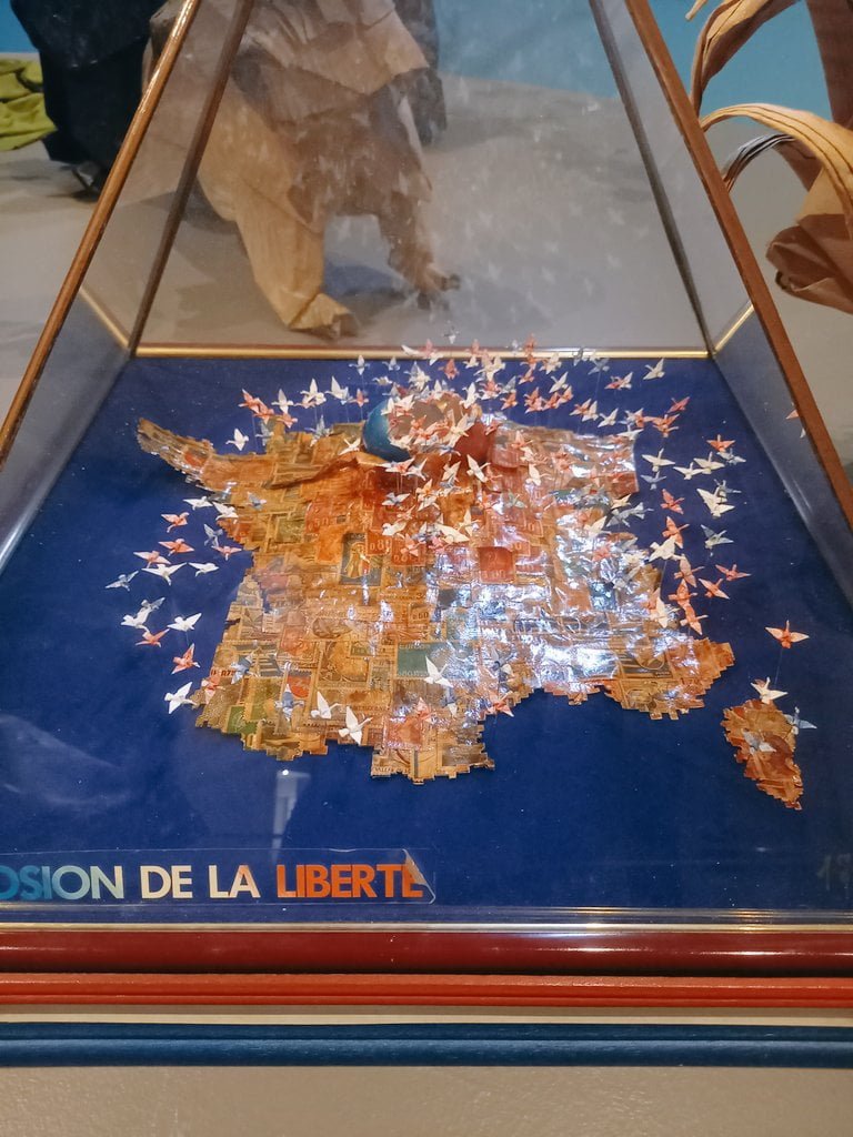

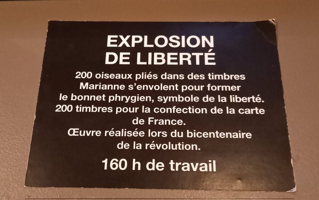
Anne L. shared these pictures last year. What could be better to celebrate Bastille Day this year? The Liberty Explosion is made with 200 stamps representing Marianne, the Symbol of the French Revolution for the Liberty, and the explosion takes the shape of the Phrygian cap.

Happy Bastille Day!
MapsintheWild Explosion de la Liberté
13 July 2024
11:00
Mappery: How goes the World?
sur Planet OSGeo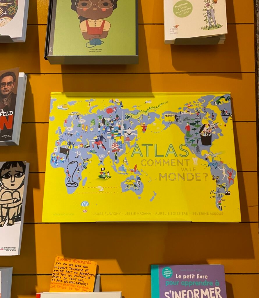

Reinder spotted this atlas in a bookshop in Lyon, “saw this Asia-Australia centered atlas cover in Librairie Passages, in Lyon, France.”

Centering the world map on Asia and Australia (which places the Americas to the east) reminds us thatthe adoption of the Prime Meridian through Greenwich was a choice by European cartographers not some inalienable geographic rule.
MapsintheWild How goes the World?
12 July 2024
19:35
KAN T&IT Blog: IOT Solution Congress en Brasil, nuestra experiencia
sur Planet OSGeo

El pasado mes de junio se llevó a cabo el IOT Solutions Congress en la ciudad de San Pablo, Brasil, donde más de 5.000 personas se reunieron para ver las soluciones más avanzadas en la industria del Internet de las Cosas (IOT).

El Internet de las Cosas es un concepto tecnológico que se resume como una red de dispositivos interconectados, ya sea a través de internet u otro tipo de redes, con el fin de enviar y recibir información en tiempo real y de forma automatizada.

Como muchas tecnologías innovadoras, el IOT tiene una amplia variedad de aplicaciones y usos, y esto se vió reflejado en la diversidad de las empresas que se acercaron al evento de San Pablo para conocer más sobre el tema. Se destacó la presencia de empresas de la industria petroquímica, minera, agrícola, de la construcción y organismos gubernamentales.

En esta ocasión KAN participó del evento con un stand y con un espacio en el Startup Stage, donde Ariel Anthieni (CEO) dió una charla sobre las aplicaciones y beneficios de los Gemelos Digitales (Digital Twins) con un enfoque particular en el monitoreo de tránsito de las ciudades.

Un Gemelo Digital es una réplica digital altamente precisa de objetos de todo tipo, desde vehículos y turbinas hasta ciudades enteras, cuyo fin es el de crear simulaciones que puedan optimizar el uso de dichos objetos. El mayor valor que otorga un Gemelo Digital es que utiliza datos reales para llevar a cabo estas simulaciones.

Primero se recolectan los datos utilizando dispositivos de telemetría IOT (sensores térmicos, caudalímetros, acelerómetros, etc.), luego se procesa esta información y finalmente se vuelca sobre el modelo virtual. Utilizando este modelo se pueden realizar diferentes tipos de simulaciones, analizar cada uno de los distintos escenarios y buscar mejoras para optimizar los recursos que se disponen.

Por ejemplo, utilizando sensores de vibración y un gemelo digital, se puede analizar el uso real de una bomba de agua, simular distintos escenarios y establecer cuándo debe hacerse el mantenimiento preventivo óptimo según los datos obtenidos.

Para el caso de las ciudades, Ariel explicó en su charla que los Gemelos Digitales permiten ayudar a los organismos gubernamentales a ver de forma anticipada el impacto que determinadas políticas públicas pueden tener en la organización de la ciudad.

Ariel lo explica en dos ejemplos sencillos: Conociendo el movimiento real de los colectivos en las ciudades, se puede simular el impacto que tendrán en sus recorridos si una avenida principal es clausurada completamente. Esto permite al gobierno buscar la reorganización óptima y desplegar eficazmente a los equipos de tránsito que llevarán a cabo la tarea.

Otro ejemplo se ve en la ciudad de Japón, donde el gobierno utiliza Gemelos Digitales para realizar simulaciones de terremotos y tsunamis para mejorar su capacidad de respuesta y recuperación ante los desastres naturales.

En conclusión, KAN cumplió con su cometido en el congreso de IOT logrando mostrar una solución vanguardista dentro de la industria IOT y dejando en claro que es una de las startups a seguir.
19:23
Free and Open Source GIS Ramblings: Trajectools 2.2 released
sur Planet OSGeo

If you downloaded Trajectools 2.1 and ran into troubles due to the introduced scikit-mobility and gtfs_functions dependencies, please update to Trajectools 2.2.

This new version makes it easier to set up Trajectools since MovingPandas is pip-installable on most systems nowadays and scikit-mobility and gtfs_functions are now truly optional dependencies. If you don’t install them, you simply will not see the extra algorithms they add:

If you encounter any other issues with Trajectools or have questions regarding its usage, please let me know in the Trajectools Discussions on Github.
13:47
WhereGroup: Volumendifferenzen, Zonenstatistik und mehr: wie Geoinformationssysteme (GIS) beim Wiederaufbau des Ahrtals helfen
sur Planet OSGeo

Geoinformationssysteme unterstützen beim Wiederaufbau im Ahrtal nach der katastrophalen Flutkatastrophe 2021. Mit QGIS machen wir Daten sichtbar für diese Herkulesaufgabe, um Maßnahmen für den Wiederaufbau abzuleiten.
11:00
Mappery: World Time in EC1
sur Planet OSGeo

Another pic from Marc-Tobias’ visit to London
MapsintheWild World Time in EC1
8:17
gvSIG Team: Acceptance Speech for the National Geographic Science Award
sur Planet OSGeo

Honorable Mr. Jesús Gómez, Undersecretary of Transport and Sustainable Mobility, distinguished authorities, ladies and gentlemen,

It is an immense honor and a profound satisfaction for me to receive, on behalf of the gvSIG Association, the first National Geographic Science Award ever given in Spain. We humbly confess that being the first to receive it, with so many deserving individuals and entities, further elevates the importance we place on this award. Additionally, it ensures that you will hear the best acceptance speech for the award to date.

This award represents an extraordinary recognition of the trajectory and dedication of a group passionate about geography, technology, and knowledge, understood as drivers of change.

Let us begin with the term that names this award, geography. Tim Marshall, in his excellent essay “Prisoners of Geography,” concluded that while geography does not dictate the development of all events, since great ideas and leaders are part of the push and pull of history, all must act within the confines that geography sets. Former U.S. President Barack Obama told us that geography was much more than putting names on a map; it was about understanding reality. Those who have listened to us over the years well know that in the gvSIG Association, we have always affirmed that reality manifests in the territory. Everything exists to the extent that it is in a place and how it relates to what is around it. Therefore, the geographic or spatial dimension of things is a fundamental attribute for managing reality. It was in the past, it will be in the future, and undoubtedly, it is in the present.

This leads us to talk about the second concept that excites us, technology. With more than two decades into the 21st century, we must all be aware that technology permeates every productive, economic, academic, and social process to the point of becoming an indispensable tool. Without fear of being wrong, I could say that there are more technological devices in this room than people. We cannot imagine that management of reality we spoke of without technology. We know that Spain and the European Union are significantly betting on science, technology, and innovation as fundamental pillars for their growth and sustainable development. For our part, in the gvSIG Association, we have always talked about technology as a strategic sector and will continue to insist on it as long as necessary. Geographic information management technologies, encompassed under the concept of geomatics, are those that allow us to analyze, understand, and manage the territory, geography.

Geomatics is applied in managing infrastructures of all kinds, in sectors such as the environment, security, energy, mobility, education, health, agriculture, tourism,… it is transversal to countless themes and applicable to countless geographies.

Thus, we should begin to be aware that being dependent on a strategic sector is a manifest weakness. Who would want our administrations, our universities, our companies, those that work in and with the territory, to be technologically dependent? Herein lies much of the importance and success of the gvSIG project: building and developing technologies for managing spatial data, its geographic dimension, with free software. Betting on technological sovereignty by promoting solutions that grant all rights and freedoms to their users. That avoid any dependence not only on technologies but on the owners of these. Not only that, the gvSIG Association has fostered its own industrial fabric, specialized in geomatics, making the Valencian Community and Spain a reference center internationally. Today, not only are gvSIG-branded technologies used worldwide, but today, Spanish companies carry out some of the largest projects related to geographic information systems around the globe. I conclude this section by reaffirming that betting on our own and free technologies can be, undoubtedly is, a strategic decision of the highest order.

We link this to the last concept related to the gvSIG Association’s activity, knowledge. And at this point, it might be worthwhile to take a look back at the history of our entity.

Let us not forget that if we are here today, receiving this important recognition, it is because one day a public administration, the Generalitat Valenciana, decided to take the first step. The gvSIG project came to light in 2004, with a first version of a software product that today is part of a complete catalog of geomatics solutions. Today, not only is it talked about, but legislation in Spain and Europe promotes reuse, sharing, interoperability among administrations, and the development of our own technologies. At the beginning of this century, it was not so. The Generalitat Valenciana not only took the first step but knew how to share the achievements with the entire international community and energize what would end up being the gvSIG Association.

Today, it continues to bet on the project, using gvSIG technologies in more and more areas, from agriculture to road safety, from industry to sustainable mobility, contributing to its development and also reusing all the technological improvements that are continuously consolidated in the project. Just last week, the Danish Agency for Digital Government published a report highlighting the Generalitat Valenciana as the main success case for the promotion of free software technology by a public administration. It spoke of gvSIG.

Therefore, this award, this recognition, is largely shared with the Generalitat Valenciana and, in particular, with its Directorate General of Information and Communication Technologies.

At the end of 2009, the gvSIG Association was born. A group of people, companies, and entities decided to scale the impact of the project. To ensure its sustainability on the one hand, to consolidate an incipient industrial fabric on the other. The premise might seem simple, but it was not easy to implement. Bringing the values of free software to the economy. Developing a new business model – a concept much talked about – based on collaboration, shared knowledge versus speculation with acquired knowledge, solidarity versus rivalry. From the dates, you may guess that we were born in the midst of a crisis, in difficult times, with few resources but with great enthusiasm. In those early years, we made the English proverb “A smooth sea never made a skilled sailor” our own. It was necessary to dream, and believing in our dreams has brought us here. After this time, we do not forget to keep dreaming.

Today, in 2024, the gvSIG Association is an entity recognized worldwide. The technology derived from a project born, let us not forget, on the periphery of Europe is used in more than 160 countries. We participate and collaborate with the main forums and organizations that promote Geographic Sciences, open knowledge, and interoperability. We have received international awards from entities such as NASA or the European Commission, which last year recognized gvSIG as the most important free software project in Europe. We have developed a suite or catalog of free technologies that allow addressing any need for information management with a geographic dimension, for any organization. We collaborate on R+D+I projects with dozens of universities, scientific publications citing the use of gvSIG are multiplying. gvSIG’s social networks have a notable influence with thousands of followers. And regarding that new business model we talked about… we have promoted the consolidation of Spanish companies and developed projects in more than 30 countries for entities of all kinds, from the United Nations to small municipalities, from large private sector energy companies to NGOs. We are, in short, an international reference center.

Our history, therefore, pivots around knowledge. Developing it to share it, to reduce asymmetries between territories, to generate quality economy, to reaffirm Antonio Machado’s saying that “in matters of culture and knowledge, you only lose what you keep; you only gain what you give.”

I want to recall an anecdote that well reflects this phrase. An example of those other values, not quantifiable, that occur around the model of knowledge, development, and business we promote in the gvSIG Association.

At an event organized by Itaipú Binacional in Foz do Iguaçu, Brazil, we were invited to give training courses both to the staff of the hydroelectric plant and, openly, to university students who wanted to attend. In the first training course, a male and a female student sitting in the front row asked the trainer (in this case, it was me) if he could put them in touch with the event organizers to ask for affordable accommodation. Then they told me their story…

At the University of Asunción, Paraguay, where they were studying, the students collectively requested the faculty to give them training in gvSIG, as they considered it a strategic investment for the country to have engineers trained in free software technologies, with all the advantages that entails. The faculty, familiar only with non-free products, refused. Among all the students, it was decided to collect funds to allow one male and one female student to make the long journey to Foz do Iguaçu, receive training, and thus, upon returning, be able to replicate the training for all the students. Today, several of those students hold responsible positions in the country.

If we have come this far, it is because many people think there can be other approaches, other ways of doing things. Therefore, to conclude, I want to thank all the people who were, are, or will be in the gvSIG project: workers, entities, communities… and especially to the colleagues for their effort and commitment, who have always put themselves at the service of the project and never put the project at their service. Our future will be full of maps, standards, algorithms, and lines of code, but above all, of people working towards a common goal. Thank you very much.
11 July 2024
11:00
Mappery: Globes holding stuff in place
sur Planet OSGeo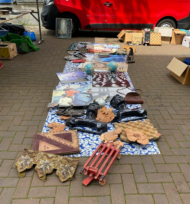

From Reinder, he spotted “Two globes at Waterlooplein-market in Amsterdam preventing the wind from blowing all the stuff away.”
MapsintheWild Globes holding stuff in place
10 July 2024
11:00
Mappery: Fantasy Islands on Forest Bikes
sur Planet OSGeo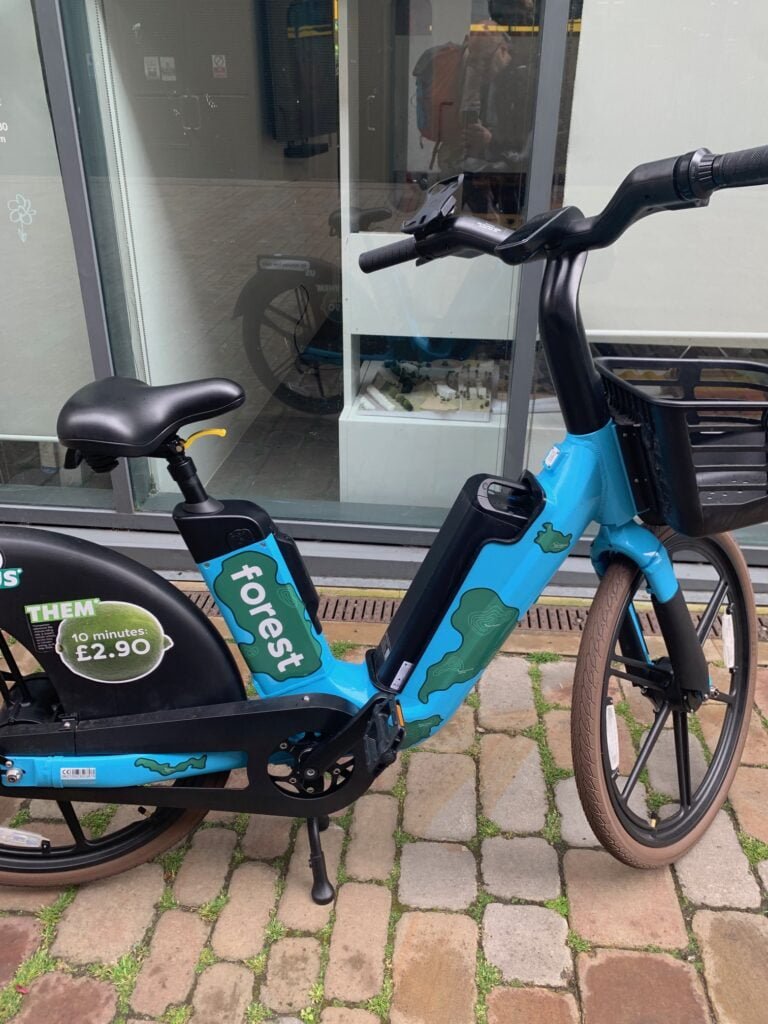

Marc-Tobias sent me these pics from his recent visit to London. Forest Bikes is a newish e-bike rental scheme in London. The bikes seem to be decorated with maps. Could they be real places, or is it a fantasy?

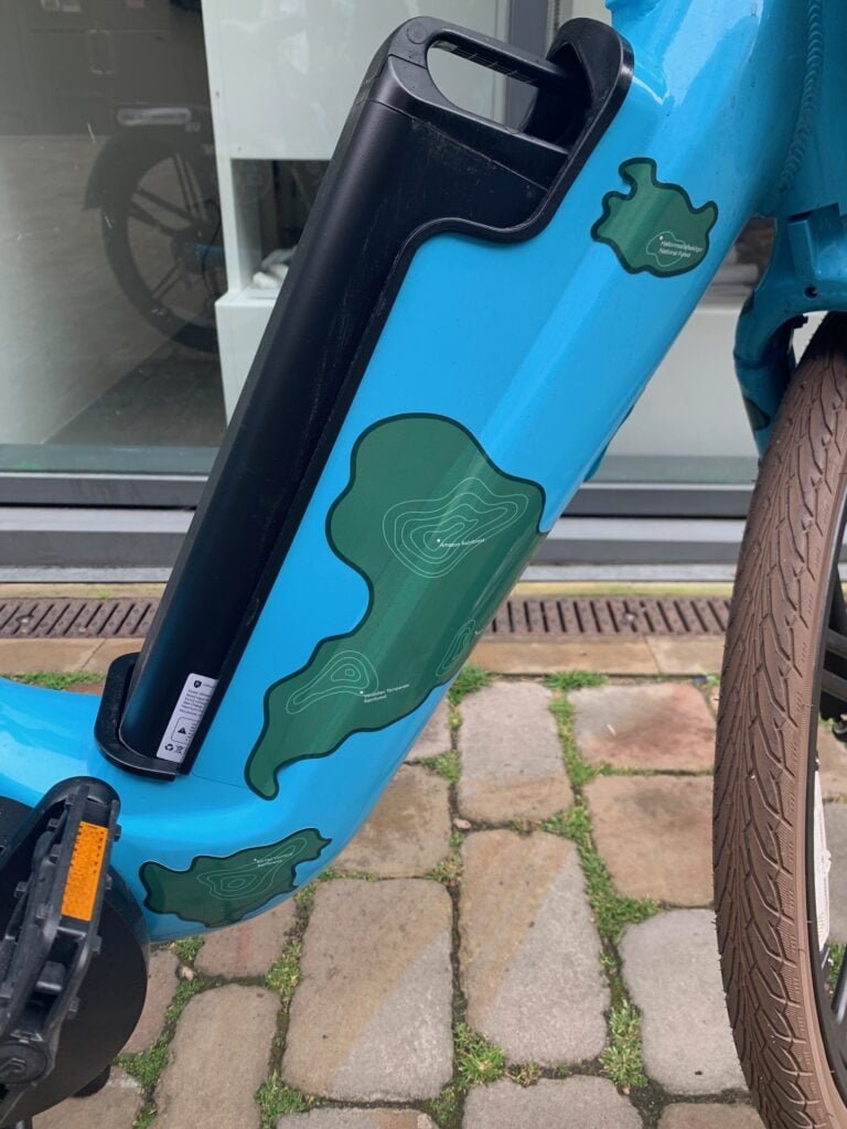
Note the contour lines

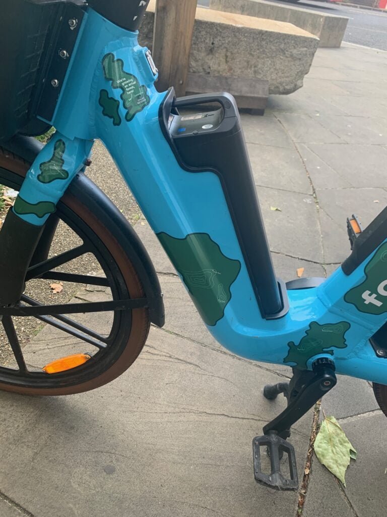
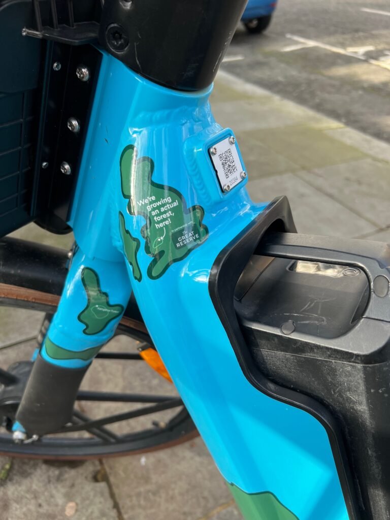
That is almost certainly the British Isles just below the handlebars.

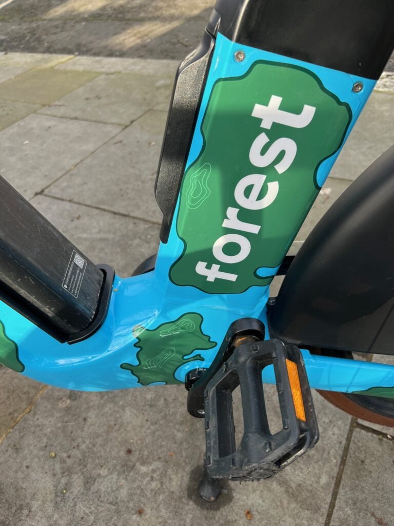
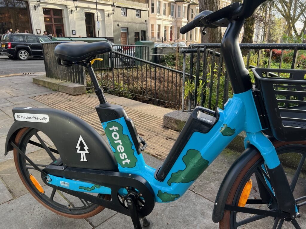
If anyone from Forest Bikes wants to comment…
MapsintheWild Fantasy Islands on Forest Bikes
09 July 2024
14:39
GeoSolutions: GeoSolutions at geOcom 2024
sur Planet OSGeo

You must be logged into the site to view this content.
11:00
Mappery: The Australian Bar
sur Planet OSGeo

Reinder sent this. You might think this is from Australia but no, it is afloat on the River Rhone. You might also be wondering why it gets featured on Mappery, well look at the zoomed in image.

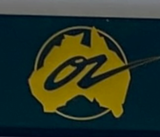
MapsintheWild The Australian Bar
08 July 2024
14:32
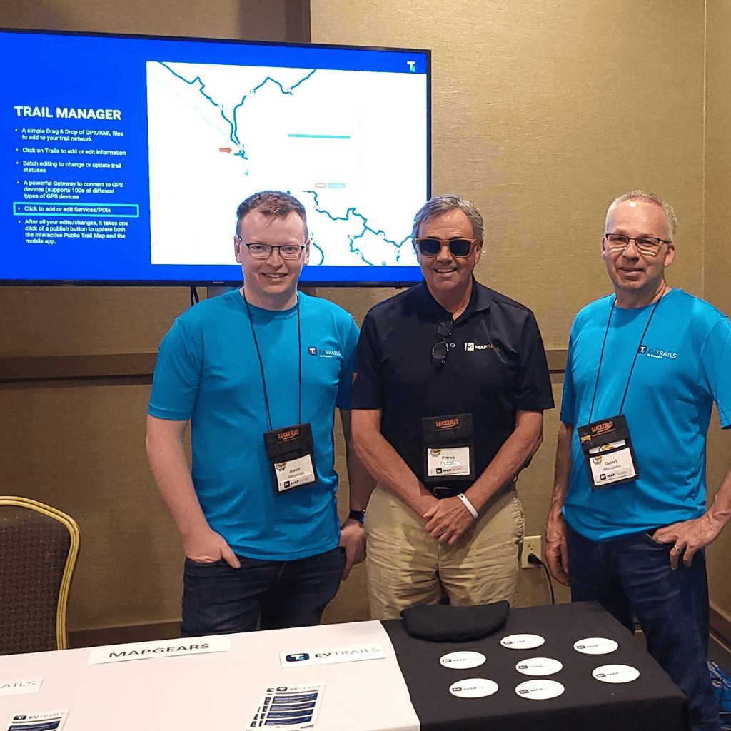
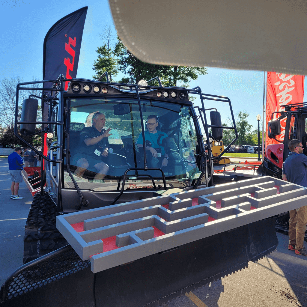
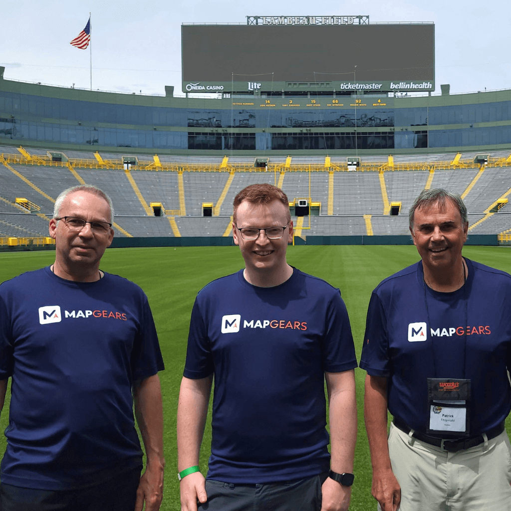
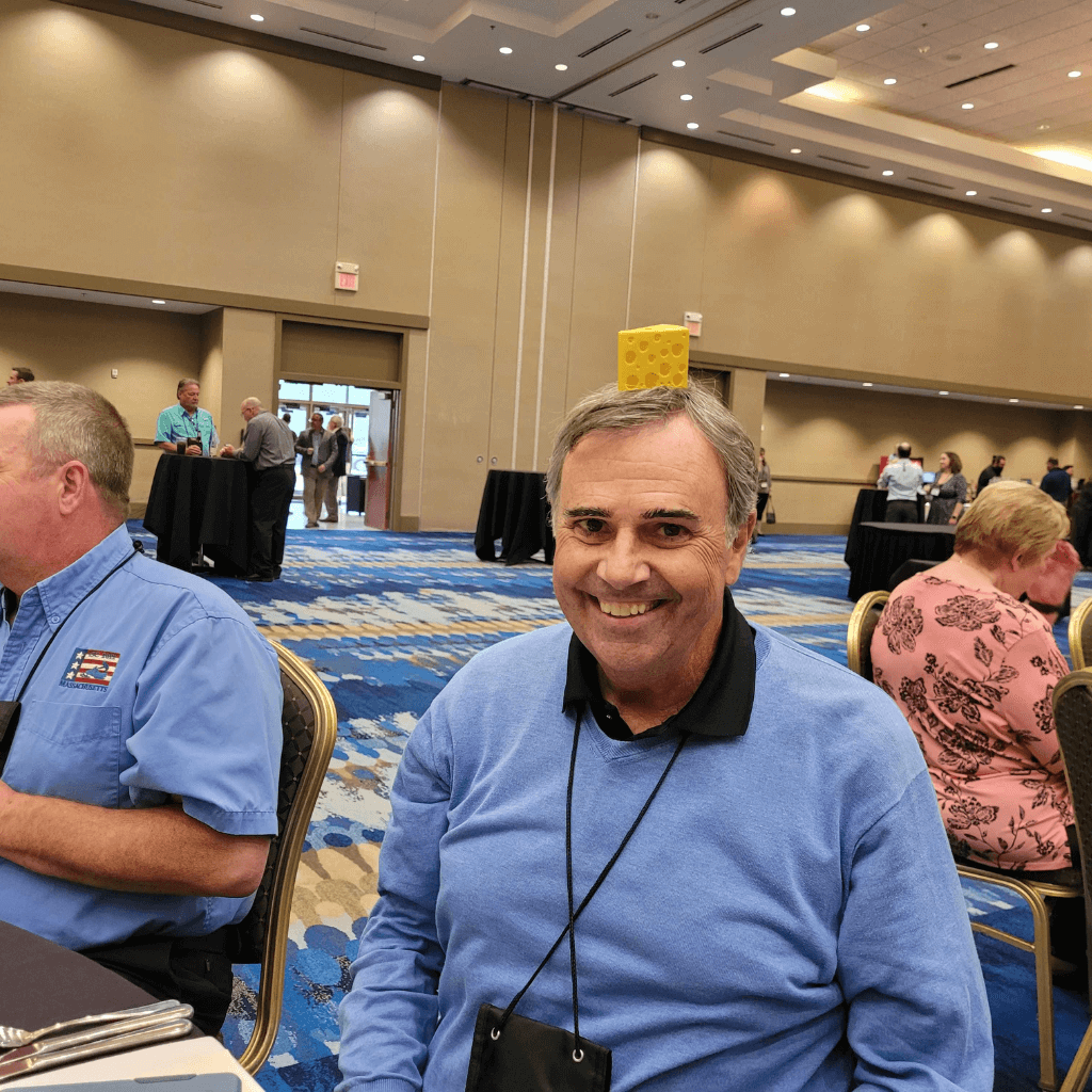
Mapgears: Recap from the 56th International Snowmobile Congress
sur Planet OSGeo

We once again attended the 56th edition of the International Snowmobile Congress, held this year in the picturesque state of Wisconsin. It was a great opportunity to engage with key figures in our industry.
As Bronze Sponsors, we reinforced our commitment to the snowmobiling community. Throughout the congress, we had meaningful face-to-face discussions with clients and explored potential partnerships with new associations interested in joining the evTrails family.
These events are always a highlight for us, enabling us to not only network within the industry but also to gain valuable insights into the needs and preferences of trail managers, particularly regarding smart mapping and related technologies.
We were thrilled to receive positive feedback from many clients who visited our booth, expressing their appreciation for our trail system and how it simplifies their daily responsibilities as trail managers. Additionally, we showcased our latest feature, Drive Up, which enhances the rider’s navigation experience through seamless driving mode integration.
The congress also provided us with invaluable client feedback on potential enhancements to our app and solutions. We returned home inspired by numerous ideas for new features that we are eager to develop and share with you.
Meanwhile, enjoy these photos of our team participating in the diverse activities at the 56th International Snowmobile Congress!

The post Recap from the 56th International Snowmobile Congress appeared first on Mapgears.
11:00
Mappery: Armidale Information Centre
sur Planet OSGeo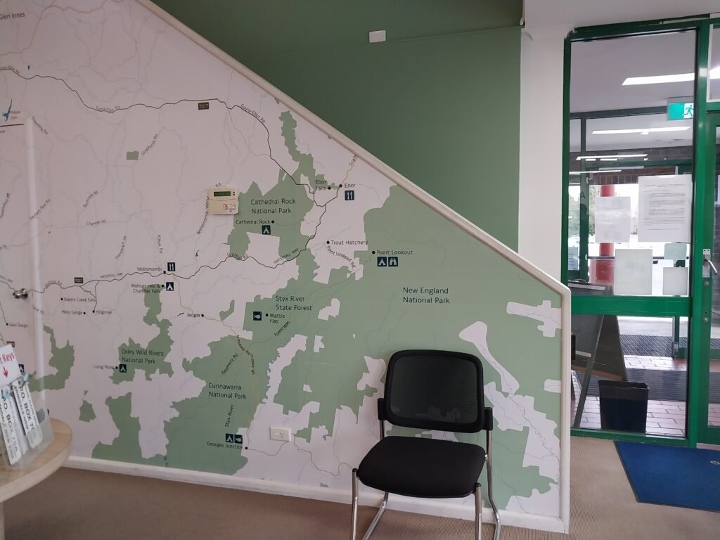

Anna Barca spotted this map on the staircase at the Armidale Information Centre. She said “The use of the staircase to display local attractions (mainly National Parks) is clever, turning a boring wall into a amazing eye-catching source of information.”

Good spot Anna and welcome to the Mappery community with your first map in the wild.
MapsintheWild Armidale Information Centre

9:04

QGIS Blog: Plugin Update – April to May, 2024

sur Planet OSGeo

Between April and May there were 33 new plugins published in the QGIS plugin repository.

Here follows the quick overview in reverse chronological order. If any of the names or short descriptions catches your attention, you can find the direct link to the plugin page in the table below:

Swiss GeoAdmin Bulk Geocoder

Bulk geocoding of Swiss building addresses using the geocoding service of geo.admin.ch, the portal of swisstopo.

EDAC Tools

A toolbox containing various Python-based tools developed by the Earth Data Analysis Center (EDAC) at the University of New Mexico.

CompareClassA

Compare two datasets of GPKG pointZ geometry based on french legislation formatting “class A”.

Stats By Polygon

This plugin creates plots for statistics of raster bands based on selected polygon feature.

UMap

This plugin enables any user to transform a stack of digital bathymetric data terrain models into a bathymetric community map.

SkyGIS

This is a plugin to download files from Skydeck, process it in QGIS and upload the results back to Skydeck portal.

Amazon Location Service

QGIS Plugin for Amazon Location Service.

CIGeoE Copy Paste Features 3D

Copy and paste features from one layer to another of the same type preserving original Z coordinate.

CIGeoE Translate To Fit To Adjacent Polygon

Do a polygon translation to the nearest polygon, by making it coincide their nearest vertices.

CIGeoE Toggle Vertex Visibility

Toggle vertex’s marker visibility.

CIGeoE Reverse Line

Reverses a selected line.

UA Coordinates Transformation

????????????? (???????????) ????????? ??????????? ???? ????? ???????? API ????????? ??????????? ??????.
Translation: Transformation of vector layer coordinates through the official API of the State Geodetic Network.

GeoBasis_Loader

GeoBasis_Loader (Open Data GeoBasisdaten).

Viper (QGIS snake clone)

Snake clone using vector layers and QGIS canvas.

jpdata

Download and load various data of Japan.

S2 Toolkit

Tools for the S2 Geometry.

PL-2000

Konwerter wspó?rz?dnych punktu uk?adu PL-ETRF2000 do uk?adu PL-2000.
Translation: PL-ETRF2000 point coordinate converter to PL-2000 system.

Luftbildfinder NRW

Find and display aerial images (German State of North Rhine-Westphalia) – Luftbilder finden und laden für NRW.

UDef-ARP Plugin

UDef-ARP for QGIS.

Route Builder

“Route Builder” is a QGIS plugin with a set of tools that calculates shortest routes in street networks using data from OpenStreetMap (OSM) and using the A* (A Star) algorithm. Users can define a region, define origin and destination points (O/D) using the coordinates collected by the plugin, these coordinates of the nodes and thus calculate the shortest route between them.

Transition-QGIS

Access a Transition transit planning server data and functionalities from QGIS.

PG service parser

View, edit or copy PG service entries.

Skråfotos

Opslag på Dataforsyningens Skråfotos.
Translation: Notice on Dataforsyningens Skråfotos.

OD_LSA_Loader (Open Data Land Sachsen Anhalt Loader)

OD_LSA_Loader (Open Data Land Sachsen Anhalt Loader) – Plugin Deprecated

QuickWebViewer

Publish your QGIS project online as web map.

ActiveBreak

ActiveBreak is a plugin for QGIS that emits messages at the top of the canvas at time intervals from the start of work, reminding the user to take an active break, take their lunch and/or reminders indicating to save their QGIS project.

QGIS Shoreline Change Analysis Tool

A plugin for Shoreline Change Analysis (SCA).

eMapTools

This plugin propose retention trees and riparian buffer zones based on ecological values.

NextGIS OGRStyle

Capture OGR Style in ONE click to paste them into a spreadsheet.

landXMLtoDB_Free

Provides LandXML to Database tools, etc, storing to PostGIS initially, later to Oracle and MS SQL.

RRR-reader

Reads RRR files.

Spatial Analyzer

Spatial Analysis Tools.

Japan GSI Point Collector

This plugin collects xyz points from gsi website. The selection should be within Japan boundary.

We would like this opportunity to highlight two plugins, Viper (QGIS snake Clone) and Active Break.

Viper allows to emulate in QGIS canvas the popular game Snake, providing a fun time and a bit of nostalgia for the “older” users. However it goes further than that, as it serves the purpose of teaching about geospatial concepts such as geometry objects (points, polygons) with their properties and methods, spatial indexing in the form of R-Tree, but also programming in QGIS, as well as other aspects.

On a more serious tone, if it can be said that, we present Active Break, a plugin that “simply” presents messages at specific time intervals, which can be personalized by the user and range from the more technical such as “save your project”, personal or motivational like quotes from hundreds of people on multiple subjects, or perhaps the most important, routinely reminders to take a break, relax or go have lunch. This considering the long hours we spent daily in front of the computer, with all the physical and mental health, as well as social implications. Congratulations on both authors!

8:00
Free and Open Source GIS Ramblings: New MovingPandas tutorial: taking OGC Moving Features full circle with MF-JSON
sur Planet OSGeo
Last week, I had the pleasure to meet some of the people behind the OGC Moving Features Standard Working group at the IEEE Mobile Data Management Conference (MDM2024). While chatting about the Moving Features (MF) support in MovingPandas, I realized that, after the MF-JSON update & tutorial with official sample post, we never published a complete tutorial on working with MF-JSON encoded data in MovingPandas.

The current MovingPandas development version (to be release as version 0.19) supports:
- Reading MF-JSON MovingPoint (single trajectory features and trajectory collections)
- Reading MF-JSON Trajectory
- Writing MovingPandas Trajectories and TrajectoryCollections to MF-JSON MovingPoint
This means that we can now go full circle: reading — writing — reading.
Reading MF-JSON
Both MF-JSON MovingPoint encoding and Trajectory encoding can be read using the MovingPandas function read_mf_json(). The complete Jupyter notebook for this tutorial is available in the project repo.

Here we read one of the official MF-JSON MovingPoint sample files:
```
traj = mpd.read_mf_json('data/movingfeatures.json')
```
Writing MF-JSON
To write MF-JSON, the Trajectory and TrajectoryCollection classes provide a to_mf_json() function:

The resulting Python dictionary in MF-JSON MovingPoint encoding can then be saved to a JSON file, and then read again:
```
import json
with open('mf1.json', 'w') as json_file:
    json.dump(mf_json, json_file, indent=4)
```
Similarly, we can read any arbitrary trajectory data set and save it to MF-JSON.

For example, here we use our usual Geolife sample:
```
gdf = gp.read_file('data/demodata_geolife.gpkg')
tc = mpd.TrajectoryCollection(gdf, 'trajectory_id', t='t')
mf_json = tc.to_mf_json(temporal_columns=['sequence'])
```
And reading again
```
import json
with open('mf5.json', 'w') as json_file:
    json.dump(mf_json, json_file, indent=4)
tc = mpd.read_mf_json('mf5.json', traj_id_property='trajectory_id' )
```
Conclusion
The implemented MF-JSON support covers the basic usage of the encodings. There are some fine details in the standard, such as the distinction of time-varying attribute with linear versus step-wise interpolation, which MovingPandas currently does not support.

If you are working with movement data, I would appreciate if you can give the improved MF-JSON support a spin and report back with your experiences.
07 July 2024
11:00
Mappery: Nikko on a Shopping Bag
sur Planet OSGeo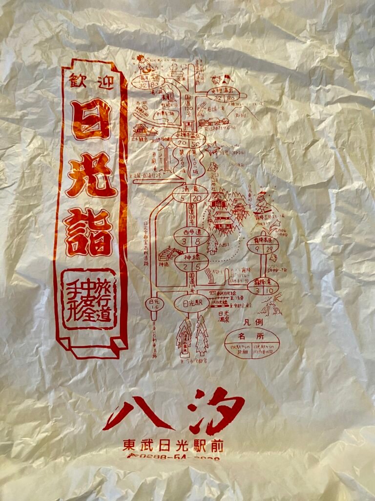

Maarten Pullen sent me this picture of a shopping bag with a map of Nikko, Japan.

“Yesterday I stumbled upon a plastic bag from Nikko, Japan, with several tourist spots on it. I wrote a little blog post (in Dutch, but can be translated) about the background of the map
[https:]

Here is a rough translation of the first part of Maarten’s blog post:

“For some time now I have been following Maps in the Wild, a collective that collects maps for aesthetic purposes in the broadest form. The core idea is that printed maps have less functional use thanks to digitization and are therefore used more for aesthetic reasons.

Or it’s just an excuse to collect a lot of eye-catching cards, which is also a good idea in my opinion.

A plastic bag from Japan came from the attic. And suddenly I realized that you can also translate it. And it also turned out to have a schematic map, showing, among other things, a bridge, temples, a ski resort and a waterfall (or Onsen?).

I got the bag in 2010 in Nikko, Japan”

And that is a perfect Map in the Wild! Thanks Maarten
MapsintheWild Nikko on a Shopping Bag
6:11
OPENGIS.ch: Rapid Mapping the Ticino Floods and Landslides with QField Rapid Mapper
sur Planet OSGeo

Pièce jointe: [télécharger]
QField Rapid Mapper is a project for the QField mobile app, which allows emergency responders, civil protection, military, and citizens to assess and report damages from natural catastrophes by quickly sharing geolocated images, videos and audio. QField Rapid Mapper offers real-time data collection, mapping and sharing to help enhance disaster response and coordination.
QField and QFieldCloud are open-source, and OPENGIS.ch is donating the needed QFieldCloud infrastructure and expertise to help map the floods in Ticino in 2024
Join the effort
OPENGIS.ch Supports Flood Mapping Efforts in Ticino
After discussing with the Protezione Civile Locarno e Valle Maggia and the Centro di Competenza per la geoinformazione (CCGEO), we are proud to announce that OPENGIS.ch is donating the necessary QFieldCloud infrastructure and dedicated projects for a rapid crowdsourcing POC to aid in mapping the 2024 floods in Ticino. This crowdsourcing initiative aims to provide essential support to professionals and volunteers working on flood and landslide assessment and recovery.

[https:]]
Empowering Response with Advanced Technology What is needed?
Photographing damaged houses and infrastructure is the most critical aspect of this mapping initiative. These images provide crucial information for assessing the extent of the damage, planning rescue and reconstruction operations, and ensuring that resources are allocated effectively. It’s also important to document any submerged or damaged vehicles, as they offer additional insights into the disaster’s impact. During these activities, it’s essential to be careful and respect the privacy and property of others, avoiding capturing license plate numbers or entering destroyed buildings without permission. Using QField Rapid Mapper can contribute to a faster and more coordinated emergency response while ensuring respect for those affected.

The QFieldCloud infrastructure enables efficient, real-time data collection and sharing, ensuring that accurate and up-to-date information is available to all stakeholders involved in the flood response. This effort underscores our commitment to leveraging technology for social good and environmental resilience.
How You Can Get Involved
1. if you don’t have a QFieldCloud account yet, sign up at [https:]]
2. fill out the quick participation form at [https:]]
By participating, you will have access to powerful tools for field data collection and can contribute valuable information to the ongoing efforts in Ticino. All the data collected will be released under the Creative Commons CC0 1.0 public domain license.
Join the Effort
Using QField and QFieldCloud, you can help create detailed maps crucial for understanding the impact of the floods and planning effective recovery strategies. Your contributions will make a significant difference in managing and mitigating the effects of this natural disaster.
Join the effort
Visit our QField Rapid Mapper project page for more information on how QField and QFieldCloud can assist in flood mapping and other field data collection projects.

Together, we can make a difference. Join us in mapping the floods in Ticino and support the community’s recovery efforts.
06 July 2024
12:00
GRASS GIS: Nix development environment and package
sur Planet OSGeo

You can now develop and run GRASS GIS with Nix A new option for creating a GRASS development environment and a unique way of running GRASS directly from the Git source code was implemented using the Nix package manager. This idea was presented by Ivan Mincik during the GRASS GIS Community Meeting in Prague. The Nix development environment provides a stable and reproducible environment for all developers and can significantly simplify the onboarding process of new contributors.
11:00
Mappery: King David’s Tower 7 – Stefan Illes 3D Map of Jerusalem
sur Planet OSGeo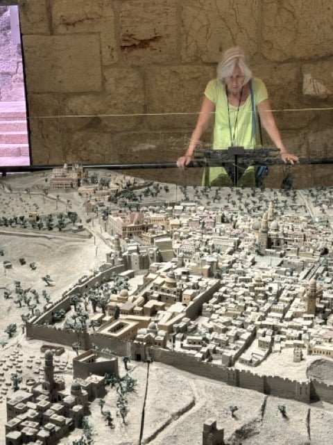

This 3D map of Jerusalem in the 19th century is massive and spectacular. It was brilliantly lit to take you through a day in the life of the city from the sun rising in the east through the day to sunset.

“Stefan Illés, an Austro-Hungarian Catholic, arrived in Jerusalem in 1864 and worked as a bookbinder at the Franciscan publishing house. Illés built a model of Jerusalem that was exhibited in the Ottoman Pavilion at the World Expo in Vienna in 1873. The model, which was highly acclaimed, was displayed throughout Germany and Switzerland. In 1878, it was purchased by a distinguished family from Geneva. Illés’s impressive model is cartographically accurate and is considered a reliable scientific source for the history and geography of Jerusalem in the 19th century.”

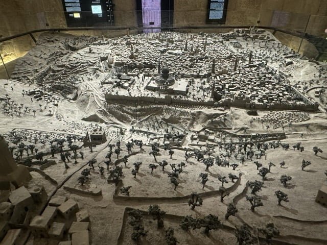
And that finishes my maps in the wild selection from King David’s Tower. There were loads more maps showing the evolution of the city through the different eras of history from the Egyptian period through Assyrian, Babylonian, Persian, Islamic, Crusader and Ottoman eras to the modern day. Well worth a visit.
MapsintheWild King David’s Tower 7 – Stefan Illes 3D Map of Jerusalem
2:00
PostGIS Development: PostGIS 3.5.0alpha2
sur Planet OSGeo
The PostGIS Team is pleased to release PostGIS 3.5.0alpha2! Best Served with PostgreSQL 17 Beta2 and GEOS 3.12.2.

This version requires PostgreSQL 12 - 17, GEOS 3.8 or higher, and Proj 6.1+. To take advantage of all features, GEOS 3.12+ is needed. SFCGAL 1.4-1.5 is needed to enable postgis_sfcgal support. To take advantage of all SFCGAL features, SFCGAL 1.5 is needed.
3.5.0alpha2
- source download md5
- NEWS
- PDF docs: en ja, zh_Hans, fr
This release is an alpha of a major release, it includes bug fixes since PostGIS 3.4.2 and new features.
05 July 2024
11:00
Mappery: King David’s Tower 6 – The Madaba Map
sur Planet OSGeo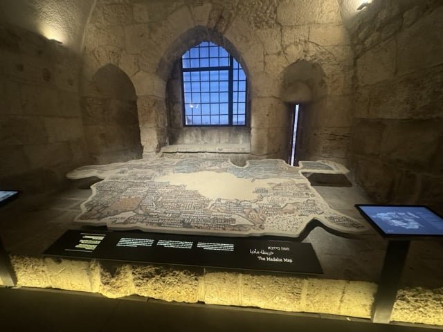

The Madaba mosaic map is one of the oldest surviving maps of Jerusalem.

“A famous Byzantine mosaic map, discovered in 1896 in the town of Madaba in Jordan. The mosaic, dated to the sixth century, emphasizes Christian sites throughout the biblical lands. The map bears the names of the sites in Greek. In the center of the map, greatly enlarged, is a map of Christian Jerusalem”

Cartographers have superimposed an image of the Madaba map onto a modern map of the old city of Jerusalem and found that the mosaic was remarkably accurate
MapsintheWild King David’s Tower 6 – The Madaba Map
04 July 2024
11:00
Mappery: King David’s Tower 5 – Jerusalem Monopoly
sur Planet OSGeo

An early version of Monopoly based in Jerusalem from the period of the British Mandate.
MapsintheWild King David’s Tower 5 – Jerusalem Monopoly
2:00
PostGIS Development: PostGIS 3.5.0alpha1
sur Planet OSGeo
The PostGIS Team is pleased to release PostGIS 3.5.0alpha1! Best Served with PostgreSQL 17 Beta2 and GEOS 3.12.2.

This version requires PostgreSQL 12 - 17, GEOS 3.8 or higher, and Proj 6.1+. To take advantage of all features, GEOS 3.12+ is needed. To take advantage of all SFCGAL features, SFCGAL 1.5.0+ is needed.
3.5.0alpha1
- source download md5
- NEWS
- PDF docs: en ja, zh_Hans, fr
This release is an alpha of a major release, it includes bug fixes since PostGIS 3.4.2 and new features.
2:00
Camptocamp: Camptocamp at GeOcom 2024
sur Planet OSGeo

Pièce jointe: [télécharger]

From June 17 to 21, Camptocamp helped organize and host the annual meeting of users and developers of the geOrchestra data infrastructure solution, to which we've been an active contributor for many years.
2:00
Camptocamp: The 3D technology serving public transport in Rennes Métropole
sur Planet OSGeo

Pièce jointe: [télécharger]

In continuation of developments linked to the Rennes Métropole territorial cooperation platform 'Coopter', Camptocamp is proud to present to you the latest application in our triptych: the TRAMBUS application.
03 July 2024
11:00
Mappery: King David’s Tower 4 – The Islamic World in the 10th Century
sur Planet OSGeo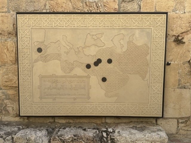

This carved stone map shows the extent of the Islamic World in the 10th Century, quite a remarkable expansion in three centuries. It’s a beautiful piece, spoilt (IMO) by the heavy black markers.
MapsintheWild King David’s Tower 4 – The Islamic World in the 10th Century
02 July 2024
15:57
GeoSolutions: GeoNode 4.3 release
sur Planet OSGeo

Pièce jointe: [télécharger]

You must be logged into the site to view this content.
11:00
Mappery: King David’s Tower 3 – Between Heaven and Earth
sur Planet OSGeo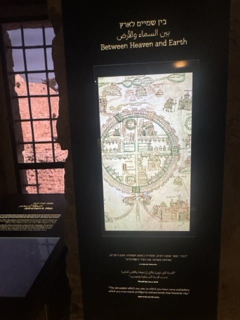

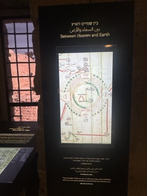
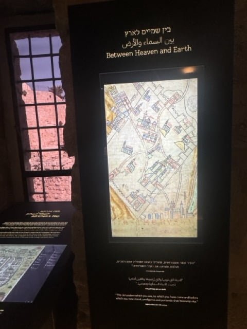
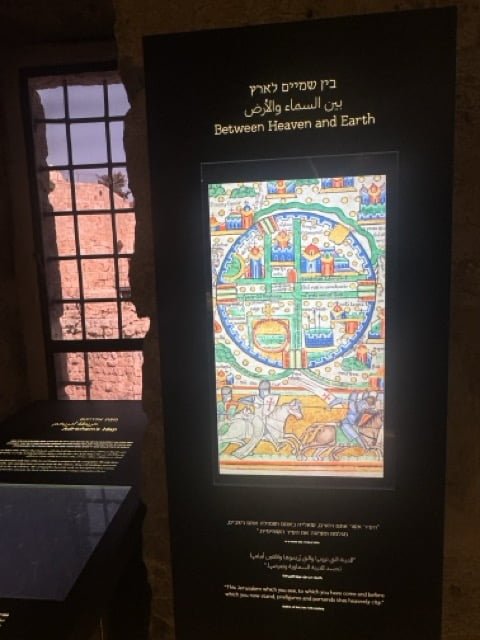
This display showed maps of Jerusalem from different periods, I like the way the maps are juxtaposed against the view through the window.
MapsintheWild King David’s Tower 3 – Between Heaven and Earth
6:04
GeoTools Team: GeoTools 28.2 Released
sur Planet OSGeo

The GeoTools team is pleased to share the availability GeoTools 28.2 : geotools-28.2-bin.zip geotools-28.2-doc.zip geotools-28.2-userguide.zip geotools-28.2-project.zip This release is also available from the OSGeo Maven Repository and is made in conjunction with GeoServer 2.22.2 and GeoWebCache 1.22.1.Update 2024-07-1: CVE-2024-36404 patch geotools-28.2-patches.zip Fixes
6:04
GeoTools Team: GeoTools 27.4 Released
sur Planet OSGeo

The GeoTools team is pleased to share the availability GeoTools 27.4 : geotools-27.4-bin.zip geotools-27.4-doc.zip geotools-27.4-userguide.zip geotools-27.4-project.zip This release is also available from the OSGeo Maven Repository and is made in conjunction with GeoServer 2.21.4.Update 2024-07-1: CVE-2024-36404 patch geotools-27.4-patches.zip Fixes and improvements
6:02
GeoTools Team: GeoTools 27.5 Released
sur Planet OSGeo

The GeoTools team is pleased to share the availability GeoTools 27.5:geotools-27.5-bin.zipgeotools-27.5-doc.zipgeotools-27.5-userguide.zipgeotools-27.5-project.zipThis release is also available from the OSGeo Maven Repository and is made in conjunction with GeoServer 2.22.3 and GeoWebCache 1.22.2.Update 2024-07-1: CVE-2024-36404 patch 
01 July 2024
21:37
KAN T&IT Blog: Expo Curitiba 2024 ¡conociendo la ciudad del futuro!
sur Planet OSGeo

Queremos compartir la experiencia de nuestro CEO, Ariel Anthieni, en Expocuritiba 2024, la Feria Internacional de Ciudades Inteligentes. Durante los días 17 al 22 de marzo, Ariel tuvo el privilegio de representar a nuestra empresa en este evento único que reunió a destacados actores en el ámbito de las ciudades inteligentes en la hermosa ciudad de Curitiba, Brasil.

Curitiba es reconocida a nivel mundial como un ejemplo de ciudad inteligente debido a sus innovadoras políticas urbanas que han transformado la calidad de vida de sus habitantes. Su eficiente sistema de transporte público, sus áreas verdes bien planificadas y su enfoque en la sostenibilidad la convierten en un modelo a seguir para otras ciudades.

Durante el evento, Ariel tuvo el honor de cruzar unas palabras con Rafael Greca, el alcalde de Curitiba. Se sorprendió gratamente por su calidez e increíble predisposición para conversar y conocer a quienes estábamos allí.

Nuestro CEO participó activamente en las diferentes actividades de la feria, incluyendo la asistencia a charlas y conferencias con reconocidos expertos en el campo de la innovación urbana, la visita a espacios temáticos y la exploración de soluciones tecnológicas innovadoras para el desarrollo sostenible de las ciudades. Tuvo la oportunidad de presentar al MapViewer, un visor digital diseñado por Kan Territory & IT para la supervisión y gestión virtual de las ciudades. Este permite monitorear y controlar diferentes aspectos de ese lugar, como el flujo del transporte público, la actividad de los centros de salud y otros servicios esenciales, a través de la recopilación y visualización de datos geoespaciales.

Ariel también destacó que el MapViewer utiliza un enfoque de catastro multifiduciario, capaz de manejar información de múltiples fuentes y tipos, como datos catastrales, topográficos y de infraestructura, proporcionando así una vista integral de la ciudad. Además, habló sobre la evolución digital de esta tecnología, introduciendo el concepto de «gemelos digitales«, que son representaciones virtuales de una ciudad. Con esta herramienta, los administradores y planificadores urbanos pueden simular escenarios hipotéticos y tomar decisiones más informadas para el desarrollo sostenible.

Sin dudas, su actividad en Expocuritiba 2024 fue una oportunidad invaluable para conocer las últimas tendencias en tecnología urbana, establecer contactos estratégicos y compartir conocimientos con otros líderes en el ámbito de las ciudades inteligentes.

Felicitamos a Ariel por su destacada participación en este evento tan significativo y esperamos seguir contribuyendo al desarrollo de ciudades más inteligentes y sostenibles en el futuro. Muchísimas gracias Lucía Bellocchio por haberlo hecho posible ¡Hasta el próximo año!
11:00
Mappery: King David’s Tower 2 – The Clover Map
sur Planet OSGeo

Bunting’s Clover Map is an archetypal map of the world from a time when only three continents were known to Europeans – Europe, Africa and Asia.

Die ganze Welt in einem Kleberblat
Woodcut Map showing three continents: Europe, Asia and Africa in the form of a clover leaf with the representation of Jerusalem in the center. America on the lower left corner.
From: Buenting, Heinrich. Itinerarium Sacrae Scripturae. (Travel book covering the entire Holy Scripture) Helmstadt, Jacobus Lucius, 1585. Part I, between pp. 4-5
[https:] FL7074006

Coincidentally I bought a wooden puzzle based on this clover map in a craft market. Apparently the solution requires over 250 moves, I am still working on it! (this is the solved state)

MapsintheWild King David’s Tower 2 – The Clover Map

9:04

QGIS Blog: Plugin Update – February to March, 2024

sur Planet OSGeo

From February to March of this year, 58 new plugins were published in the QGIS plugin repository.

Here follows the quick overview in reverse chronological order. If any of the names or short descriptions catches your attention, you can find the direct link to the plugin page in the table below:

Indonesian Multi-scaled Grid System

This plugin automate the determination of Indonesia’s Environmental Support and Capacity.

NDVI to Variable Nitrogen Application Map

This plugin was developed for producing variable nitrogen application maps based on index (e.g. NDVI, EVI) values.

Dynamic Flow

Compare two datasets of GPKG pointZ geometry based on french legislation formatting “class A”.

Stats By Polygon

Dynamic Flow is a QGIS plugin to estimate the spatio-temporal 3D gradient flow from the point observation of the attributes values such as aggregated cell-phone mobility data.

On-the-Fly-Shortest-Path

Interactively find shortest path between points over a line network and calculate the Fiber Loss Budget of a fiber optic network (backbone or FTTH)

SMODERP2D

This plugin calculates hydrological and erosion processes on individual plots or small catchments.

Multifilter

Filter multiple layers

NDVI and EVI Index Calculator

This plugin calculates NDVI and EVI index from Sentinel 2 B02, B04 and B08 Bands.

GeoZone

QGIS plugin for adding and modifying zone data in compliance with the GeoZone schema, facilitating sharing with partners or uploading to a central web repository.

CIGeoE Mirror View

Add one or more panels synchronized with the main panel.

SIOSE Tools

Herramientas SIOSE.

RioGIS 2

Export to WinCan.

Clasificación de redes hídricas

Este plugin clasifica las redes hídricas por medio de una etapa de enriquecimiento y otra de lógica difusa. Advertencia: Versión experimental, algunos procesos pueden ser largos de aplicar.

AutoStyler

Apply QML style files to new layers. QML files are stored in {qgis_home}\Styles directory. QML files will be applied to a vector layer when the QML file’s basename is found as a substring of the new layer’s name. QML files will be applied to a raster layer when the QML file’s label token is found as a substring of the new layer’s name. The label token is raster_style_{label}.qml.

Delta Shares

With this plugin you can load data from delta shares

Simple ETL

A simple ETL for spatial data

Flood Path Finder

Developed with Python by Emerson N. Santos – 2024

MongoDB Layer

This plugin gives the possibility to create a layer from MongoDB datasource

Power Pin PL

Plugin eksportuje pinezk? do serwiów typu geoportal. Pin to popular polish and world maps portal. Plugin export pin to popular geoportal like serives

Mineral Exploration Web Services

This plugin connects your QGIS User Profile to many openly hosted web services related to mineral exploration. These include Country and State geological surveys that provide mapped geology and data such as mineral occurence locations, geophysics, geochemistry etc.

OrfeoToolbox Provider

OrfeoToolbox Processing provider.

MitiConnect

MitiConnect integrates ecological connectivity in mitigation hierarchy based on landscape graphs.

Compare_attributes

Compare Attributes

Geo Cluster

This plugin allows you to cluster different territorial scopes.

Estonian Oblique Aerial Photographs

Get the oblique aerial photographs of Estonia at the clicked location on the map

Two distances intersection

Get the intersection of two distances (2D cartesian)

Show Corona CAST by click

This plugin opens a webpage showing the Corona CAST map in the clicked coordinates on the canvas

Roll

Design and analysis of 3D seismic survey geometries

moniQue

Monoplotting oblique images with uncertainty estimation.

Modular Layout Grid Guides

This plugin creates a modular layout grid for print layouts

easyPlugin

Plugin which creates a simple QGIS plugin templates ready for install, editing and testing

Samon

Saisie monoscopique sur la BD Ortho

SADI Processor

A plugin to Process Standardized Agricultural Drought Index.

SciPy Filters

Filter collection implemented with SciPy

Data Validator

Prototype for vector data validation

ZUMbox

Urban planning related tools

UA_NGO_PDF_Parser

This plugin parse pdf files with NGO data and create table with result

Marine Tools

Tools for marine habitat mapping

Map tools

QGIS plugin for little helpers in map production

Style Exporter

Plugin export styles of selected layers to individual file with name same as layers name.

Aino

AI assistant to download data from OSM

gis3d

This plugins generates a 3D model based on the inputs

Zonal Exact Extract

Zonal Statistics of rasters using Exact Extract library

Verkeersborden

Import dutch traffic signs.

NVDB Les

NVDB (Norwegian Administration Road Database) it’s a plugin to analyse and manipulate road objects, like (road references, trees, light poles, traffic signs, construction area, smart devices like IP Camera, tunnels, bridges, etc)

Fluvial Corridor Toolbox

CIGeoE Reshape Features 3D

Reshape a feature in 3D

Pixel Purity Index

Pixel Purity Index algorithm

C-GEO Wizualizacja GML demo

Wtyczka wczytuje oraz wizualizuje dane EGiB, GESUT, BDOT500 zapisane w plikach GML.

pqkmeans-clustering

This clustering algorithm is a quantized version of the K-Means algorithm that is memory and computationaly more efficient.

HedgeTools

HedgeTools is a plugin for QGIS designed to extract and characterize hedges, aiming to streamline field efforts by providing information about hedge health.

PyXel_Sync

SmartSDI

Wtyczka SmartSDI (Geo-System) PL: Pobieranie danych wektorowych: dzia?ki, budynki, adresy EN: Downloading vector data for Poland: parcels, buildings, addresses

Quick_search

Environmental Data Retrieval

Environmental Data Retrieval QGIS plugin

DigiAgriApp

Plugins to work with DigiAgriApp server

QTalsim

This plugin creates hydrological response units (HRUs) suitable for Talsim ( [www.talsim.de] ) and allows users to connect to a Talsim DB.

RubberSheetingEtc

Provides Rubber Sheeting and Two Point Transformations, storing to PostGIS, Oracle and MS SQL. The Rubber Sheeting algorithm uses supplied Shift Vectors and calculates the weighted average shift from the 10 nearest Shift Vectors. The Two Point Transformations handles themes with and without a CRS.

30 June 2024
14:52
Free and Open Source GIS Ramblings: New interactive trajectory plots for MovingPandas & experiments on their interpretation using ChatGPT 4o
sur Planet OSGeo

With the release of GeoPandas 1.0 this month, we’ve been finally able to close a long-standing issue in MovingPandas by adding support for the explore function which provides interactive maps using Folium and Leaflet.

Explore() will be available in the upcoming MovingPandas 0.19 release if your Python environment includes GeoPandas >= 1.0 and Folium. Of course, if you are curious, you can already test this new functionality using the current development version.

This enables users to access interactive trajectory plots even in environments where it is not possible to install geoviews / hvplot (the previously only option for interactive plots in MovingPandas).

I really like the legend for the speed color gradient, but unfortunately, the legend labels are not readable on the dark background map since they lack the semi-transparent white background that has been applied to the scale bar and credits label.

Speaking of reading / interpreting the plots …

You’ve probably seen the claims that AI will help make tools more accessible. Clearly AI can interpret and describe photos, but can it also interpret MovingPandas plots?
ChatGPT 4o interpretations of MovingPandas plots
Not bad.

And what happens if we ask it to interpret the animated GIF from the beginning of the blog post?

So it looks like ChatGPT extracts 12 frames and analyzes them to answer our question:

Its guesses are not completely off but it made up the facts such as that the view shows “how traffic speeds vary over time”.

The problem remains that models such as ChatGPT rather make up interpretations than concede when they do not have enough information to make a reliable statement.
11:00
Mappery: King David’s Tower 1 – Adrichem’s Map
sur Planet OSGeo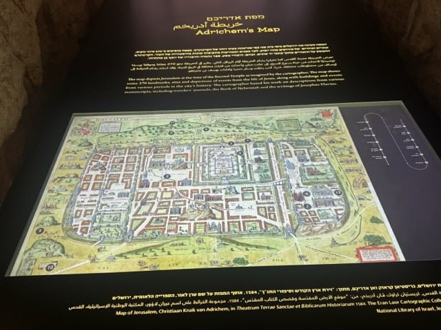

While we were in Israel we spent some time in Jerusalem, friends suggested that we visit the new museum about Jerusalem in King David’s Tower. It is a fantastic museum in an ancient location which reflects the different influences in the city over three millenia. Amongst the many exhibits were a lot of maps, ancient, modern, interactive, over the next few days I will share a few.

Adrichem was a 16th century Dutch cartographer, this map of Jerusalem shows remarkable detail

“A map of Jerusalem created by the Dutch cartographer Christiaan van Adrichem in 1584. In this beautifully illustrated map are drawings that represent events and figures from the Old and New Testaments. Toward the center of the map the Jewish Temple can be seen together with a drawing of the High Priest, the altar and the vessels used in the Temple. To the right of the Temple is the Royal Palace, pictures of King Solomon on his throne, and even Bathsheva bathing on her rooftop. Other drawings on the map, such as the Via Delarosa and images of the Crucifixion, depict the Christian history of Jerusalem.”
[https:]

MapsintheWild King David’s Tower 1 – Adrichem’s Map
29 June 2024
11:00
Mappery: Globe Escape Alert!
sur Planet OSGeo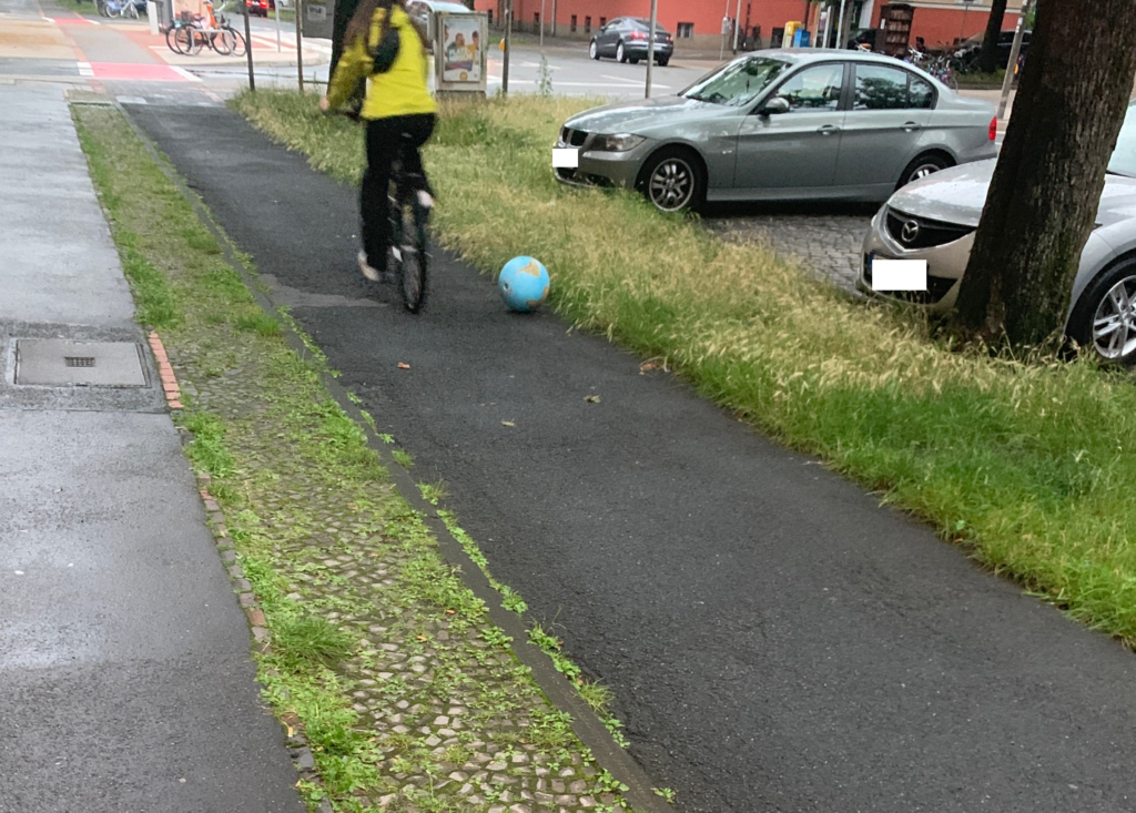

Marc-Tobias spotted this little globe that had set out on a journey to freedom starting in Hannover, I wonder where it will end up?

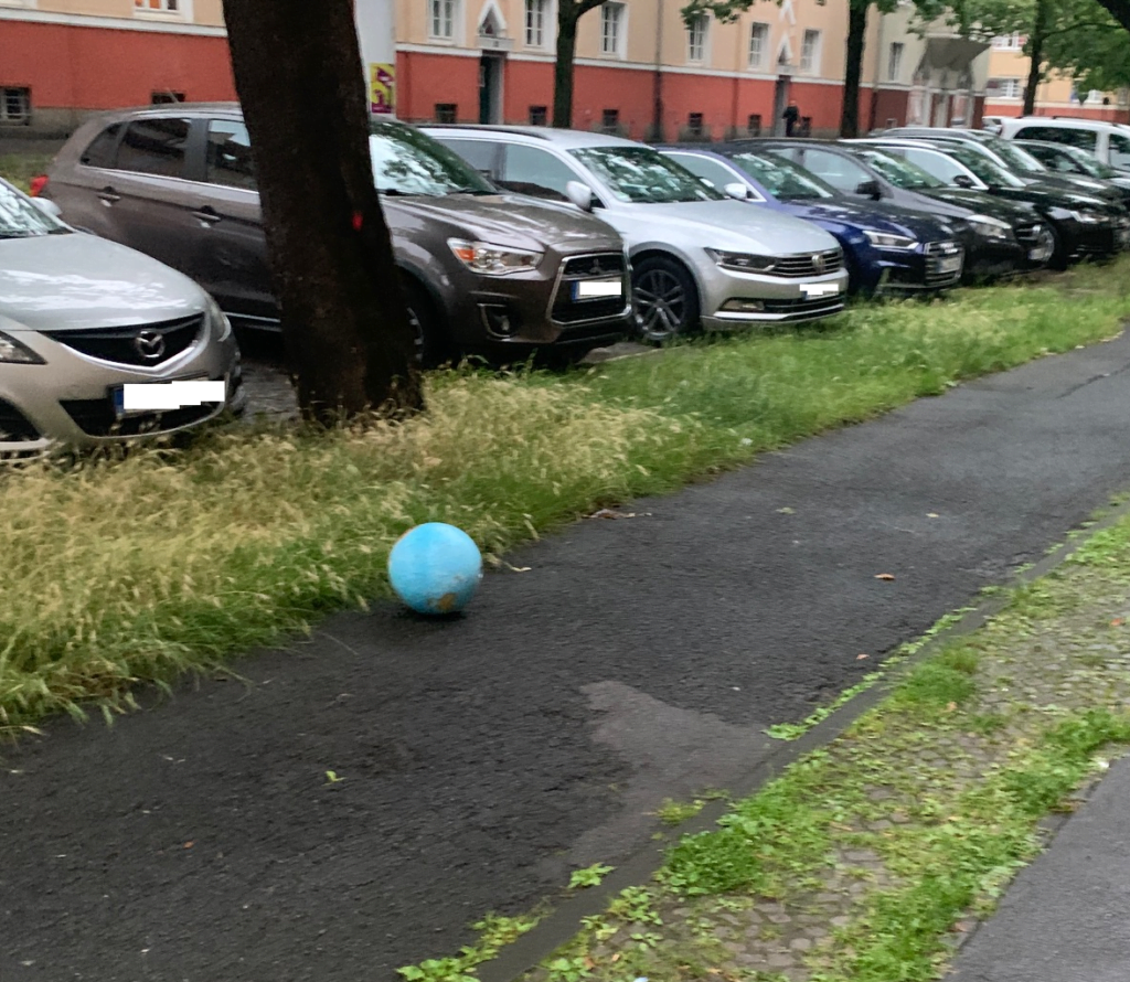
Good luck little globe

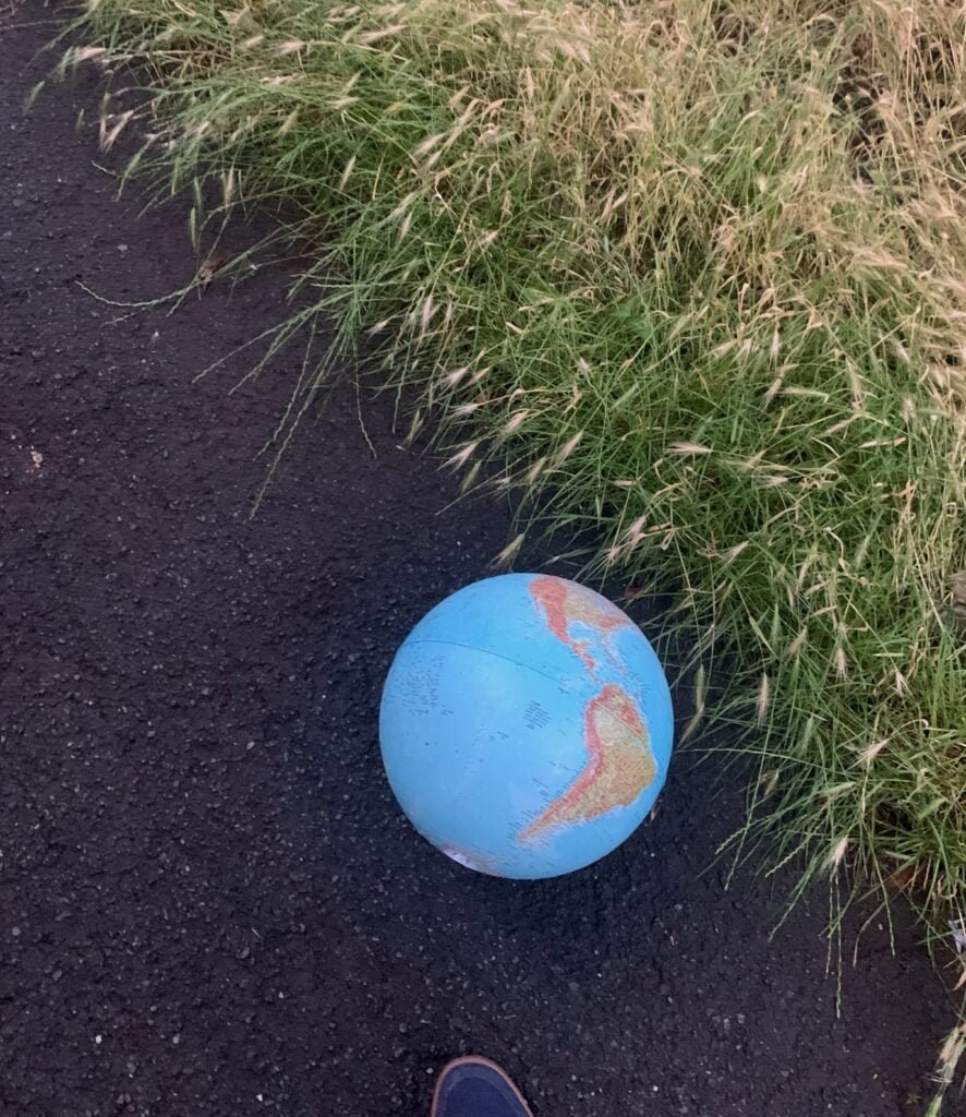
MapsintheWild Globe Escape Alert!
28 June 2024
16:13
gvSIG Team: Discurso de aceptación del Premio Nacional de Ciencias Geográficas
sur Planet OSGeo

Excmo. Sr. Jesús Gómez, Subsecretario de Transportes y Movilidad Sostenible, distinguidas autoridades, señoras y señores

Es para mi un inmenso honor y una profunda satisfacción recibir, en nombre de la Asociación gvSIG, el primer Premio Nacional de Ciencia Geográficas que se otorga en España. Humildemente confesamos que ser los primeros en recibirlo, con la cantidad de personalidades y entidades que lo merecen, todavía acrecienta más la importancia que le damos a este galardón. Por otro lado, nos asegura que escucharan el mejor discurso de aceptación del premio de los habidos hasta la fecha.

Este galardón supone un reconocimiento extraordinario a la trayectoria y dedicación de un colectivo apasionado por la geografía, la tecnología y el conocimiento, entendidos como motores de cambio.

Empecemos por el término que da nombre a este galardón, la geografía. Tim Marshall, en su excelente ensayo «Prisioneros de la Geografía» concluía que si bien la geografía no dicta el desarrollo de todos los acontecimientos, puesto que las grandes ideas y líderes forman parte del tira y afloja de la historia, todos ellos deben actuar dentro de los confines que marca la geografía. El ex-presidente de los Estados Unidos, Barack Obama, nos decía que la geografía era mucho más que poner nombres en un mapa, que se trataba de entender la realidad. Los que nos han escuchado durante estos años bien saben que en la Asociación gvSIG siempre hemos afirmado que la realidad se manifiesta en el territorio. Todo existe en la medida que está en un lugar y en cómo se relaciona con lo que tiene alrededor. Por tanto, la dimensión geográfica o espacial de las cosas es un atributo fundamental para gestionar la realidad. Lo fue en el pasado, lo será en el futuro y, sin duda, lo es en el presente.

Lo que nos lleva a hablar del segundo concepto que nos apasiona, la tecnología. Con más de dos décadas en el S.XXI todos debemos ser conscientes que la tecnología impregna todo proceso productivo, económico, académico y social hasta el punto de convertirse en una herramienta imprescindible. Sin miedo a equivocarme podría afirmar que en esta sala hay más aparatos tecnológicos que personas. No podemos imaginar esa gestión de la realidad de la que hablábamos sin tecnología. Sabemos que España y la Unión Europea están apostando significativamente por la ciencia, la tecnología y la innovación como pilares fundamentales para su crecimiento y desarrollo sostenible. Por nuestra parte, en la Asociación gvSIG, siempre hemos hablado de la tecnología como un sector estratégico y seguiremos insistiendo mientras sea necesario. Las tecnologías de gestión de información geográfica, englobadas bajo el concepto de geomática, son aquellas que ni más ni menos nos permiten analizar, entender y gestionar el territorio, la geografía.

La geomática se aplica en la gestión de infraestructuras de todo tipo, en sectores como el del medio ambiente, la seguridad, la energía, la movilidad, la educación, la sanidad, la agricultura, el turismo,… es transversal a infinidad de temáticas y aplicable a infinidad de geografías.

Siendo así, deberíamos empezar a ser conscientes de que ser dependientes de un sector estratégico es una debilidad manifiesta. ¿Quién querría que nuestras administraciones, nuestras universidades, nuestras empresas, aquellas que trabajan en y con el territorio, fueran dependientes tecnológicamente? Aquí radica en gran parte la importancia y éxito del proyecto gvSIG, construir y desarrollar tecnologías para gestión de datos espaciales, de su dimensión geográfica, con software libre. Apostando por la soberanía tecnológica mediante el impulso de soluciones que otorgan todos los derechos y libertades a sus usuarios. Que evitan cualquier dependencia ya no de tecnologías, sino de los dueños de estas. No solo eso, la Asociación gvSIG ha impulsado un tejido industrial propio, especializado en geomática, convirtiendo a la Comunidad Valenciana y a España en un centro de referencia a nivel internacional. Hoy día no solo las tecnologías marca gvSIG se utilizan en todo el mundo, hoy día empresas españolas llevan a cabo por todo el planeta algunos de los más grandes proyectos relacionados con los sistemas de información geográfica. Concluyo este apartado reafirmando que apostar por tecnologías propias y libres puede ser, sin duda lo es, una decisión estratégica de primer orden.

Enlazamos con el último concepto que relacionaba con la actividad de la Asociación gvSIG, el conocimiento. Y en este punto quizá valga la pena hacer un recorrido por la historia de nuestra entidad.

No hay que olvidar que si hoy estamos aquí, recogiendo este importantísimo reconocimiento, es porque un día una administración pública, la Generalitat Valenciana, decidió dar el primer paso. El proyecto gvSIG ve la luz en 2004, con una primera versión de un producto de software que hoy forma parte de un completo catálogo de soluciones de geomática. Hoy no solo se habla, sino que se legisla, en España y en Europa, a favor de la reutilización, de compartir, de interoperar entre administraciones y de desarrollar tecnologías propias. En los comienzos de este siglo no era así. La Generalitat Valenciana no solo dio el primer paso, sino que supo compartir los logros con toda la comunidad internacional y dinamizar lo que acabaría siendo la Asociación gvSIG.

Hoy día sigue apostando por el proyecto, utiliza las tecnologías gvSIG en cada vez más áreas, desde agricultura a seguridad vial, desde industria a movilidad sostenible, contribuyendo a su desarrollo y, también, reutilizando todas las mejoras tecnológicas que continuamente se consolidan en el proyecto. Sin ir más lejos, la semana pasada La Agencia de tecnologías del gobierno danés publicó un informe en que ponía como principal caso de éxito del impulso de una tecnología en software libre por una administración pública a la Generalitat Valenciana. Hablaba de gvSIG.

Por tanto, este premio, este galardón, es en gran medida compartido con la Generalitat Valenciana y, en particular, con su Dirección General de Tecnologías de la Información y Comunicación.

A finales de 2009 nació la Asociación gvSIG. Un conjunto de personas, empresas, entidades decidimos escalar el impacto del proyecto. Para garantizar sus sostenibilidad por un lado, para consolidar un tejido industrial incipiente por otro. La premisa puede parecer sencilla, pero no era fácil de implementar. Llevar los valores del software libre a la economía. Desarrollar un nuevo modelo de negocio – un concepto del que tanto se habla – basado en la colaboración, en el conocimiento compartido frente a la especulación con el conocimiento adquirido, en la solidaridad frente a la rivalidad. Por las fechas ya intuirán que nacimos en plena crisis, en momentos complicados, con escasos recursos pero con mucha ilusión. Esos primeros años hicimos nuestro el proverbio inglés de «que ningún mar en calma hizo experto a un marinero». Era preciso soñar y creyendo en nuestros sueños hemos llegado hasta aquí. Pasado este tiempo, no nos olvidamos de seguir soñando.

Hoy, en 2024, la Asociación gvSIG es una entidad reconocida en todo el mundo. La tecnología derivada de un proyecto nacido, no lo olvidemos, en la periferia de Europa se utiliza en más de 160 países. Participamos y colaboramos con los principales foros y organizaciones que promueven las Ciencias Geográficas, el conocimiento abierto y la interoperabilidad. Hemos recibido premios internacionales de entidades como la NASA o la Comisión Europea, que el pasado año reconoció a gvSIG como el proyecto de software libre más importante de Europa. Hemos desarrollado una suite o catálogo de tecnologías libres que permiten abordar cualquier necesidad de gestión de información con dimensión geográfica, para cualquier organización. Colaboramos en proyectos de I+D+i con decenas de universidades, se multiplican las publicaciones científicas que citan el uso de gvSIG. Las redes sociales de gvSIG tienen una influencia notable con miles de seguidores. Y en relación a ese nuevo modelo de negocio del que hablábamos… hemos impulsado la consolidación de empresas españolas y desarrollado proyectos en más de 30 países para entidades de todo tipo, de Naciones Unidas a pequeños ayuntamientos, de grandes empresas privadas del sector de la energía a ONGDs. Somos, en definitiva, un centro de referencia a nivel internacional.

Nuestra historia por tanto pivota alrededor del conocimiento. Desarrollarlo para compartirlo, para reducir asimetrías entre territorios, para generar economía de calidad, para reafirmar a Antonio Machado cuando decía que «en cuestiones de cultura y saber, solo se pierde lo que se guarda; solo se gana lo que se da».

Quiero recordar una anécdota que refleja bien esta frase. Un ejemplo de esos otros valores, no cuantificables, que ocurren alrededor del modelo de conocimiento, desarrollo y negocio que impulsamos en la Asociación gvSIG.

En un evento organizado por Itaipú Binacional en Foz do Iguaçu, en Brasil, se nos invitó a dar cursos de formación tanto al personal de la central hidroeléctrica como, de manera abierta, a aquellos universitarios que quisieran asistir. En el primer curso de formación, un alumno y una alumna que se situaban en primera fila, preguntaron al formador (en este caso, era yo) si podía ponerles en contacto con los organizadores del evento para preguntar por un hospedaje económico. Entonces me contaron su historia…

En la Universidad de Asunción, Paraguay, donde ellos cursaban estudios, los alumnos en su conjunto habían solicitado al profesorado que les dieran formación en gvSIG, ya que consideraban que era una apuesta de futuro para el país el contar con ingenieros formados en tecnologías de software libre, con las ventajas que ello tiene. El profesorado, conocedor solo de productos no libres, se negó. Entre todos los estudiantes se decidió hacer una colecta que permitiera a uno y a una de ellos hacer el largo viaje a Foz do Iguaçu, formarse y así, al regresar, poder replicar la formación para todo el alumnado. Hoy día varios de esos alumnos tienen puestos de responsabilidad en el país.

Si hemos llegado hasta aquí es porque hay mucha gente que piensa que puede haber otros enfoques, otras maneras de hacer las cosas. Por eso, para acabar quiero agradecer a todas las personas que estuvieron, están o estarán en el proyecto gvSIG, trabajadores, entidades, comunidades… y muy especialmente a los compañeros y compañeras por su esfuerzo y compromiso, siempre se han puesto al servicio del proyecto y nunca han puesto el proyecto a su servicio. Nuestro futuro estará llenos de mapas, estándares, algoritmos y líneas de código, pero sobre todo de personas trabajando por un objetivo común. Muchas gracias.
14:36
GIScussions: W3W – It’sGetting.Better.AlltheTime
sur Planet OSGeo
Excuse the corny title and associated video but I couldn’t resist it.

What3Words’s accounts for 2023 have just been published and the cynics who have doubted W3W’s commercial model were confounded by the outstanding progress that the company has made in 2023. Here are a few highlights to save you reading through 45 pages.
- Revenues surged by 28% to break through the £1m barrier for the first time
- Employee numbers fell from 152 to 128
- Admin expenses fell by 54% to £21.7m – “primarily driven by the reduction in consumer acquisition activities and the fair value adjustment relating to convertible loan notes” (That’s less advertising and what might be described as “debt swap magic”)
- The loss for the year fell by 48% to £16.4m
- The Directors consider W3W to be a going concern with cash and cash equivalents of £14.8 and term deposits of £12.8 at the end of the year which gives them well over a year’s runway at current revenue and expenditure levels.
- Raised £6.9m via a cash convertible loan instrument – it’s good to see that smart investors with a long term horizon continue to support W3W
- W3W has cumulative losses of £136m so when they do start to make profits in the near future the tax authorities will not be a beneficiary for several years.
You might think that summary was a bit dry so I asked a friendly AI to give me a slightly more positive view:
What3Words absolutely smashed it in 2023!
Revenue rockets! They blasted past the £1 million mark for the first time, a whopping 28% increase. That’s impressive growth for any company, but for a young innovator like What3Words, it’s a sign of things to come!

Leaner, meaner, revenue machine! While the team size trimmed down slightly, they achieved amazing things. Admin expenses plummeted by 54%! This financial wizardry involved cutting back on marketing spend and some clever financial maneuvering. Talk about efficiency!

Losses slashed in half! The deficit shrunk by a mighty 48%, proving their business model is tightening its grip.

The future’s bright! With over £27 million in the bank and a year’s worth of runway at current spending, What3Words is well-positioned for continued success.

Smart money says “Yes!” Investors are clearly bullish! A cool £6.9 million was raised through a fancy loan thingy (cash convertible loan instrument, for those keeping score). This shows that big thinkers recognize the long-term potential of What3Words.

Taxman blues? Not anymore! With a hefty pile of past losses, What3Words gets a tax break for years to come. That’s more money to fuel their innovative ideas!

In short, 2023 was a phenomenal year for What3Words. They’re growing, they’re efficient, and they’ve got the financial backing to keep pushing boundaries. If you’re looking for a company on the rise, What3Words is a shining star!

PLEASE NOTE THAT THE ABOVE REVIEW IS NOT A FINANCIAL RECOMMENDATION!
12:39
GeoCat: GeoCat Bridge for ArcGIS Pro has arrived!
sur Planet OSGeo
We are super excited to report that the very first official release of GeoCat Bridge for ArcGIS Pro is now available to all our customers.
GeoCat Bridge for ArcGIS® Pro is an add-in for Esri’s leading desktop GIS application, that allows you to publish your maps and metadata to your open data space.

All users can try GeoCat Bridge for free using our demo server as your playground. You no longer need a trial license to discover the full potential of Bridge.

GeoCat Live or Enterprise customers can contact us to activate their complimentary GeoCat Bridge licenses, or migrate their old GeoCat Bridge for ArcMap license.

Some of the key features of GeoCat Bridge for ArcGIS Pro version 1.0 are:
- Publish ArcGIS feature and raster layers as GeoCat Map or GeoServer WMS, WFS, and WCS layers
- Publish layer metadata to a GeoCat Find or GeoNetwork catalog service (ISO 19139)
- Automatic links between the map and catalog service(s) to increase discoverability
- Automatic group layers
- Automatic metadata thumbnail generation, so the record looks good
- Convert ArcGIS layer symbology to SLD with GeoServer vendor options
- Preview generated SLD and export it as a style package, containing any referenced PNG or SVG images
- Browse GeoServer workspace contents and add WMS layers on-the-fly
- Create and delete GeoServer workspaces
- Publish whole maps as a workspace or publish selected layers to existing workspaces
For instructions and an overview of all the features this version has to offer, consult our documentation.
Try now Order now
Try out or buy GeoCat Bridge for ArcGIS Pro now and let us know what you think! We value your feedback and suggestions.

Stay tuned for future updates, as more features and improvements will be added!

The post GeoCat Bridge for ArcGIS Pro has arrived! appeared first on GeoCat bv.
12:24
Adam Steer: Cartography as code: Cartopy
sur Planet OSGeo

This story calls back a long way to my mapping roots. I started out making scientific maps using the venerable Generic Mapping Tools (GMT) to plot bathymetry, ship tracks, sampling stations. Almost two decades later, I’m still making maps with code! However, this time it’s in Python – with some helpers. Here’s the end product… Read More »Cartography as code: Cartopy
11:00
Mappery: New York, mosaic
sur Planet OSGeo

Matt Malone spotted this fantastic mosaic-tiled map of NYC ? at LaGuardia Airport during his first trip there last October. As a geographer, he said he was required to take a picture and share it.
MapsintheWild New York, mosaic
27 June 2024
11:30
WhereGroup: Mapbender-Anwendungen einfach direkt aus QGIS heraus erstellen
sur Planet OSGeo

Mit unserem neuen Plugin für QGIS ist es nun möglich, QGIS-Desktop-Projekte mit nur ganz wenigen Schritten als WMS und gleichzeitig als Mapbender Anwendungen zu veröffentlichen.
11:00
Mappery: Western Hemisphere
sur Planet OSGeo

This came from Moritz Schillinger

“This map painting is from David Hardy showing the western hemisphere (artist name Le Suisse Marocain – website [https:]] ). Not sure if it’s a Map in the Wild, it’s hardly recognizable. “

No worries about eligibility Moritz, our standards are very flexible.
MapsintheWild Western Hemisphere
26 June 2024
11:00
Mappery: The Geographic Center of the United States is at …
sur Planet OSGeo

Ander Andersen is another new contributor. He kicks off with marker for the geographic center of the US. UK readers please forgive the US spelling of what should be “centre” but given the location I thought I should follow their convention.

Of course anything that claims to be the geographic centre of a country or polygon is going to prompt some discourse in the geo community. The marker has Lat 39 degrees 50 minutes, Long 98,35 but, as you might expect Wikipedia has a whole article about the different options – this marker is at the centre of the 48 contiguous states and located Lebanon, Kansas

If you include Alaska and Hawaii the centre shifts to Lat 44,58, Long 103,56 which is north of Belle Fourche in South Dakota.
MapsintheWild The Geographic Center of the United States is at …
25 June 2024
11:00
Mappery: Berlin, Schoneberg
sur Planet OSGeo

What a fantastic station signage! Marc-Tobias sent me this which he spotted on his way home from a recent Geomob Berlin event.

Note that it includes coordinates
MapsintheWild Berlin, Schoneberg
6:43
OPENGIS.ch: QGIS Swiss Locator 3.0 brings elevation profiles and vector tiles
sur Planet OSGeo

Swiss elevation profiles
Get high-precision elevation profiles in QGIS right from Swisstopo’s official profile service, based on swissALTI3D data!
Swiss elevation profiles are available with QGIS 3.38.
Thanks to this integration, you can take advantage of existing QGIS features, such as exporting 2d/3d features or distance/elevation tables, as well as displaying profiles directly in QGIS layouts.

Tip: Swiss elevation profiles will be available as long as the Swiss Locator plugin is installed and active. Should you need to turn Swiss elevation profiles off to create other profiles with your own data, go to the Plugin manager and deactivate the plugin in the meantime.
For developers
We’re paving the way for adding custom elevation profiles to QGIS. For that, we’ve added a QGIS profile source registry so that plugin developers can register their own profile sources (e.g., based on profile web services, just like we did here) and make them available for QGIS end users. The registry is available from QGIS 3.38. It’s your turn!

Thanks to the QGIS user group Switzerland for funding this feature!
Swiss vector tiles base maps
Loading Swiss vector tiles is now easier than ever. Just go to the locator bar, type the prefix “chb” (add a white space after that) and you’ll get a list of available and already styled Swiss vector tiles layers. Some of them will even load grouped auxiliary imagery for reference.

Vector tiles will be loaded at the bottom of the QGIS layer tree as base maps, so you will see all your data on top of them.

Vector tiles are optimized for local caching and scale-independent rendering. This also makes it a perfect fit for adding it to your QField project.

There are a couple of different vector tile sets available:
leichte-basiskarte Light base map
Similar to the leichte-basiskarte layer, but using an older version of the data source and adjusted styles.
leichte-basiskarte-imagery (with WMTS sublayer) Imagery base map (with WMTS sublayer)
This layer is similar to the leichte-basiskarte-imagery layer, but it uses an older version of the data source and adjusted styles.
Base map
See the official services documentation for details on data sources and styles.
Fixes
Thanks to your feedback, we’ve also fixed some issues. Don’t hesitate to reach out to us at GitHub if you’d like to suggest or report something related to the Swiss Locator plugin.

Happy (and now more powerful) mapping!
24 June 2024
11:00
Mappery: Norrebro Collection
sur Planet OSGeo

Rollo shared this water bottle with a street map
MapsintheWild Norrebro Collection

8:38

QGIS Blog: Plugin Update – December 23? to January 24?

sur Planet OSGeo

Between December 2023 and January 2024, 45 new plugins were published in the QGIS plugin repository. On top of those, we also included another 4 from the last week of November.

Here follows the quick overview in reverse chronological order. If any of the names or short descriptions catches your attention, you can find the direct link to the plugin page in the table below:

OpenLog

High performance drillhole visualization QGIS module supporting 3D, cross-section, and log views.

Benthic Terrain Modeler

Analyzes benthic terrain for the purposes of classifying surficial seafloor characteristics that may be used in studies of benthic habitat, geomorphology, prediction of benthic fish species distribution, marine protected area design, and more

QAnnAGNPS

This plugin integrates the AnnAGNPS model into QGIS

QSU2

QSU2 for CFD simulations

Autofill Attributes

Simple screen to fill your attributes table automatically.

Eurostat downloader

This plugin can be used to get data using the Eurostat API.

VectorToDBLoader

Loads Active Vector Themes to PostGIS, Oracle and MS SQL

MunsellRGB

Munsell code to sRBG conversion.

WFS Styler Plugin

Set a WMS style to a WFS layer

CIGeoE Rename Attachment Attribute

Rename attachment attribute of selected field on all features

QGIS2API-CNIG

Complemento que crea un visualizador cartográfico con el contenido del lienzo de QGIS

Data Sources Panel

Panel/dock with overview of layer data sources

GeoFA

Gratis og let adgang til GeoFA (Geografiske Fagdata i GeoDanmark) i QGIS.
Free and easy access to GeoFA (Geographical Professional Data in GeoDanmark) in QGIS.

Co-Traveler

Co-Traveler discovery tools.

CoGEOS

This plugin enables the user to automatically extract shorelines and compute shoreline change rates.

Geovita GIS Processing provider

This plugin adds different Geovita custom processing algorithms to QGIS

CAV

Este plugin realiza cálculos, comparações e análises estatísticas do volume e área de uma cota específica em um modelo digital de terreno.

Whitebox Workflows for QGIS

Provides access to Whitebox Workflows within QGIS

Y!maptool?Yahoo! JAPAN YOLP Web API

Yahoo!JAPAN?YOLP Web API??????????????????????????????????????????Web???? by Yahoo! JAPAN ?? [https:] This plugin allows the user to displays the location of search results using Yahoo!JAPAN YOLP Web API.You can search by zip code.

QgisToUGCS

A Plugin to create UGCS missions from GPKG layers. This is made for drone users that want to lead AreaScan for a drone-line inspection

Infra3D plugin

This plugin is an integration of the Infra3D application with QGIS

CZML Moving Objects

This plugin creates CZML files for moving objects described as points

Layer Tree Tools

Sorts and groups nodes in layer tree, takes layer tree snapshots

Localisation Grand Lyon

Suite d’outils de localisation utilisés pour les logiciels métiers QGIS de la Métropole Grand Lyon.

FIM

Forest Inventory and Monitoring

Point Cloud Filter Slider

GUI panel to change values in simple query builder filter for point clouds.

Dokumente verknüpfen

With this Plugin documents can be connected to objects. It is designed for sewer system inspection data.

Bunting Labs AI Vectorizer

Intelligent autocomplete for vectorizing raster maps.

CIGeoE Pacman

Resolve the intersection of 2 polygons by removing the overlapped area in the second polygon.

GSI-AddressSearch

??????API?????????????????????????????????????????????????????????????API?? [https:] plugin allows the user to search for a address and get its coordinates using GSI API.

Riverscapes Viewer

Explore symbolized Riverscapes projects

Feature Z Setter

Sets the Z value of each new/edited feature to a specific value, based on a DEM layer plus an offset.

BrandGIS

BrandGIS Ledningsstöd och geografisk lägesbild vid brand i skog och mark.

Oemc Plugin

This plugin provides easy access to OEMC STAC catalog

Swedigarch Geotools

Urbantracer

Urbantracer creates urbanized area polygon over a street map.

Geohash Expressions Plugin

This plugin adds four expression functions to work with geohash in the field calculator

QMetadataLayerHISPANIA

Complemento para visualizar y agregar metadatos a las capas.

Mesh Flow

Tool to extract flow from hydraulic model results contained in a mesh layer.

QRiS

QGIS Riverscapes Studio (QRiS)

SAGis Excel Export

Plugin öffnet einen vereinfachten Excel-Export-Dialog

SAGis ALKIS Suche

Plugin zum Einbinden und Durchsuchen einer ALKIS-Datenbank

LandXML to Mesh

Conversion of LandXML to Mesh and vice versa

QuickCopy

Click and Copy WKT.

Style to text

Converts stylefiles to csv-files

R-ABLE plugin

R-ABLE plugin, developed within the EUHubs4Data project, providing access to the web services on agricultural land.

Python Module Manager

Show all the installed packages (distributions); Show modules in a selected package; Install a package/packages; Load a module and get the version.

PDD-QGis Tool

Tool to download and visualize datasets from Plataforma de Datos by Itrend.

Project Full Text Search

This plugin generates a full text search index containing all attributes of all layers of a loaded project. The user then can use a single text-input field to search within all available attributes.

23 June 2024
11:00
Mappery: You are on the Plate
sur Planet OSGeo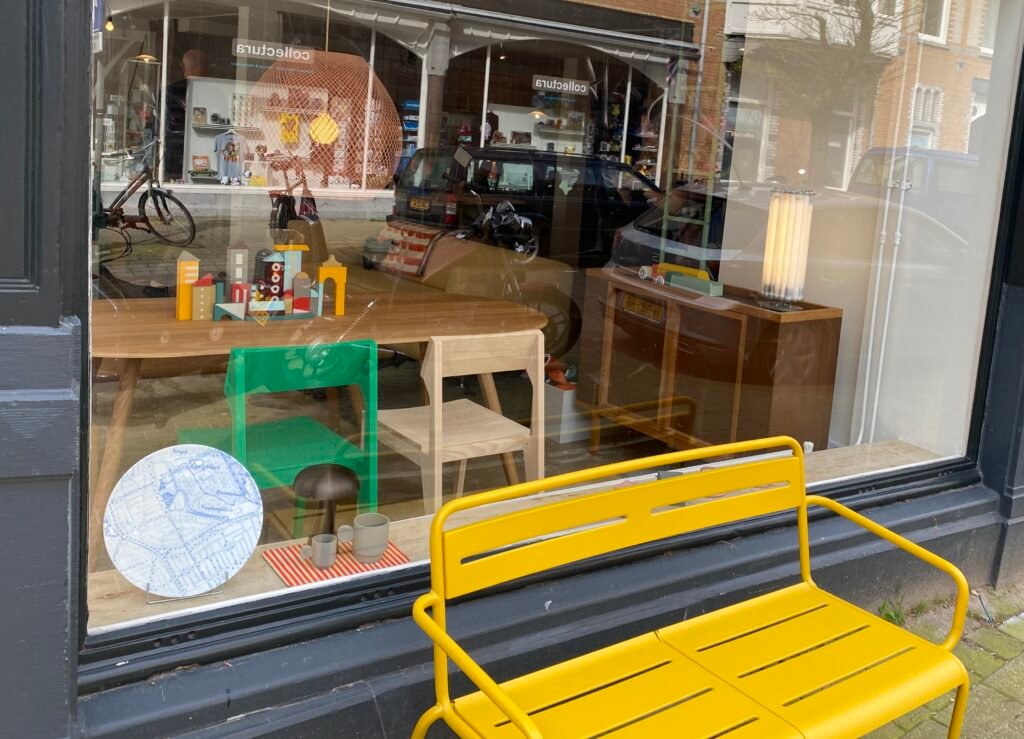

Reinder spotted this plate in a shop window in The Hague.

“Shop window, Piet Heinstraat, The Hague, Netherlands. The spot where one can see this little scene is actually on the plate, down on the right hand side.”

MapsintheWild You are on the Plate
22 June 2024
11:00
Mappery: Map Mannequin in Paris
sur Planet OSGeo

Moritz Schillinger joins the club of Maps in the Wild contributors with his first post of this superb map mannequin.

“Last weekend in Paris I discovered a map in the wild myself. I found these artworks in the art center “59 Rivoli”, a former squat which now hosts really cool (temporary) art studios.

The map mannequin here is from Isabelle Marty (artist’s name @i.m.arty – Instagram). What I can see is that she’s wearing pieces of France, Ireland and the Netherlands. “

Welcome to the club Moritz, keep them coming!

MapsintheWild Map Mannequin in Paris

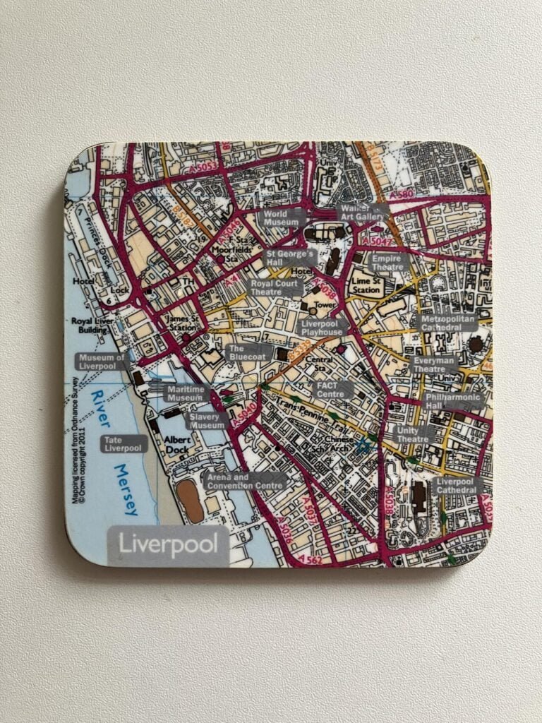
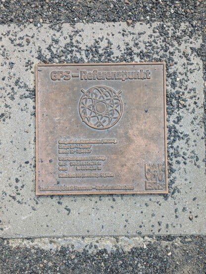
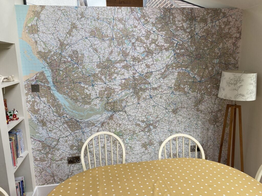
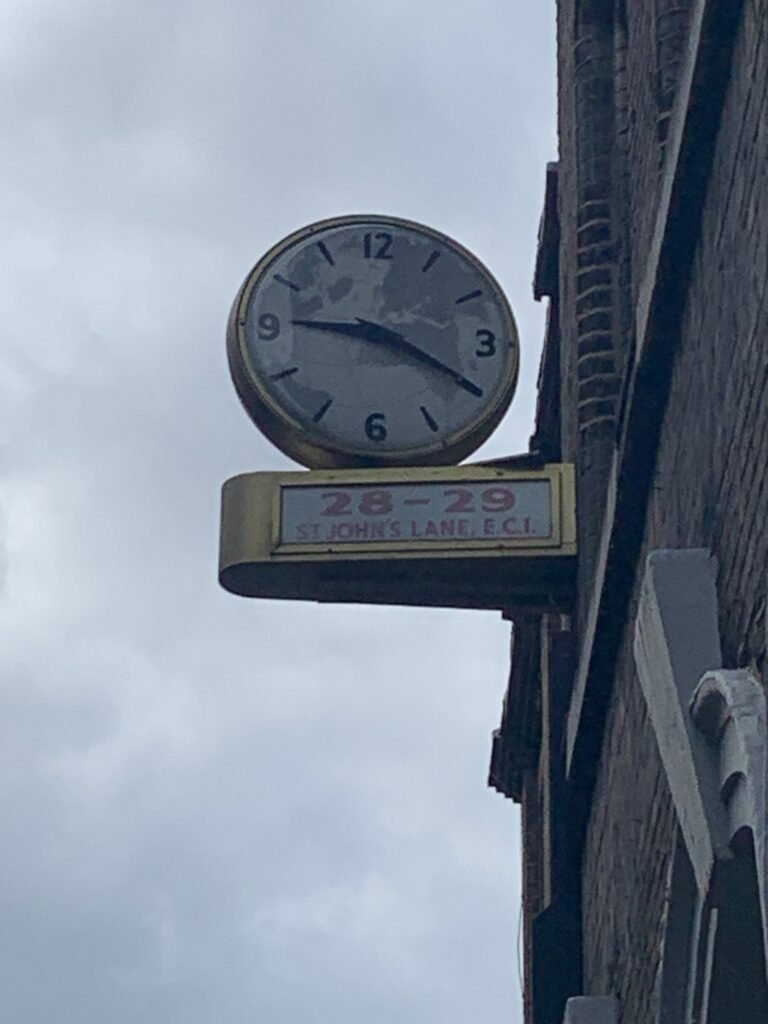
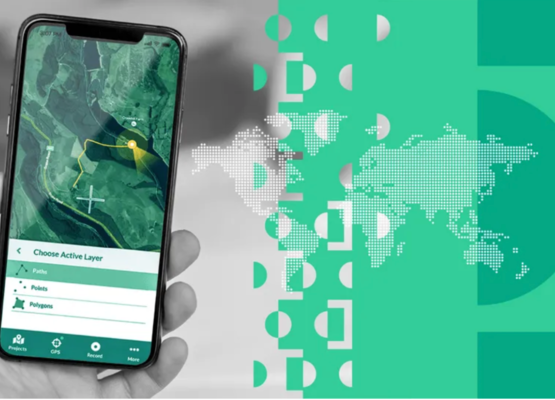
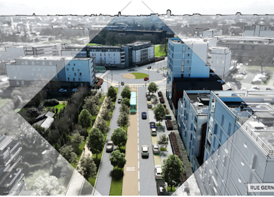Sauter à la page: 1 2 3 ... 6

← Open Geospatial Consortium (OGC) Parcell'air →

Communauté	Ressources	L'emploi	Le marché	L'association	Fils RSS
Forum Blogs Wiki Planet Sites amis	Agenda Biblio Fiches AMO-CNIG Paris PCGIS Téléchargements	Offres d'emploi Banque de CV Formations Démarche Métiers	Geo-Entreprises Geo-Communiqué Appels d'offres	L'association Qui sommes-nous ? Nous aider Bienfaiteurs Partenaires Historique Statuts	Tout le site Job Géomatique Services GeoBlogs ...	Faire un don Mentions légales

Le portail francophone de la géomatique

Canaux

Planet OSGeo

Pièce jointe: [télécharger]

Pièce jointe: [télécharger]

Pièce jointe: [télécharger]

Pièce jointe: [télécharger]

Pièce jointe: [télécharger]